
SLIDE 1
Gram-Schmidt algorithm
Aim lecture: We use the theory of last lecture to give an algorithm for finding
- rthonormal bases.
As usual in this lecture F = R or C & V is an F-space equipped with an inner product (·|·).
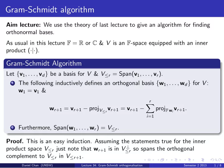
Gram-Schmidt Algorithm
Let {v1, . . . , vd} be a basis for V & V≤r = Span(v1, . . . , vr).
1
The following inductively defines an orthogonal basis {w1, . . . , wd} for V : w1 = v1 & wr+1 = vr+1 − projV≤r vr+1 = vr+1 −
r
- i=1
projF wivr+1.
2
Furthermore, Span(w1, . . . , wr) = V≤r.
- Proof. This is an easy induction. Assuming the statements true for the inner
product space V≤r just note that wr+1 is in V ⊥
≤r so spans the orthogonal
complement to V≤r in V≤r+1.
Daniel Chan (UNSW) Lecture 34: Gram-Schmidt orthogonalisation Semester 2 2013 1 / 8