
SLIDE 1
Gradient for Cross-Entropy Loss with Sigmoid
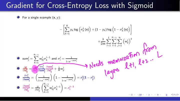
For a single example (x, y): − K
- k=1
yk log
- σL
k (x)
- + (1 − yk) log
- 1 − σL
k (x)
- + λ
2m
L
- l=1
sl−1
- i=1
sl
- j=1
- wl
ij
2 suml
j = sl−1
- k=1
wl
kjσl−1 k
and σl
i = 1 1+e−suml
i
∂E ∂wl
ij
= ∂E
∂σl
j
∂σl
j
∂suml
j
∂suml
j
∂wl
ij
+ λ
m wl ij ∂σl
j
∂suml
j
=
- 1
1+e−suml
i
1 −
1 1+e−suml
i
- = σl
j(1 − σl j) ∂suml
j
∂wl
ij
=
∂ ∂wl
ij
sl−1
- k=1
wl
kjσl−1 k
- = σl−1
i