Google matrix analysis of directed networks Lecture 2 Klaus Frahm - - PowerPoint PPT Presentation

Google matrix analysis of directed networks

Lecture 2 Klaus Frahm

Quantware MIPS Center Universit´ e Paul Sabatier Laboratoire de Physique Th´ eorique, UMR 5152, IRSAMC

• A. D. Chepelianskii, Y. H. Eom, L. Ermann, B. Georgeot, D. Shepelyansky

Networks and data mining Luchon, June 27 - July 11, 2015

Contents

Spectrum of Wikipedia . . . . . . . . . . . . . . . . . . . . 3 Eigenvectors of Wikipedia . . . . . . . . . . . . . . . . . . 4 Chirikov Standard map . . . . . . . . . . . . . . . . . . . . 9 Perron-Frobenius matrix for chaotic maps . . . . . . . . . . 10 Eigenvalues . . . . . . . . . . . . . . . . . . . . . . . . . 12 Complex density of states . . . . . . . . . . . . . . . . . . 13 Eigenvectors . . . . . . . . . . . . . . . . . . . . . . . . . 14 Diffuson modes . . . . . . . . . . . . . . . . . . . . . . . . 19 Extrapolation of eigenvalues . . . . . . . . . . . . . . . . . 22 Strong chaos . . . . . . . . . . . . . . . . . . . . . . . . . 23 Separatrix map . . . . . . . . . . . . . . . . . . . . . . . . 26 Phase space localization . . . . . . . . . . . . . . . . . . . 27 References . . . . . . . . . . . . . . . . . . . . . . . . . . 28 2

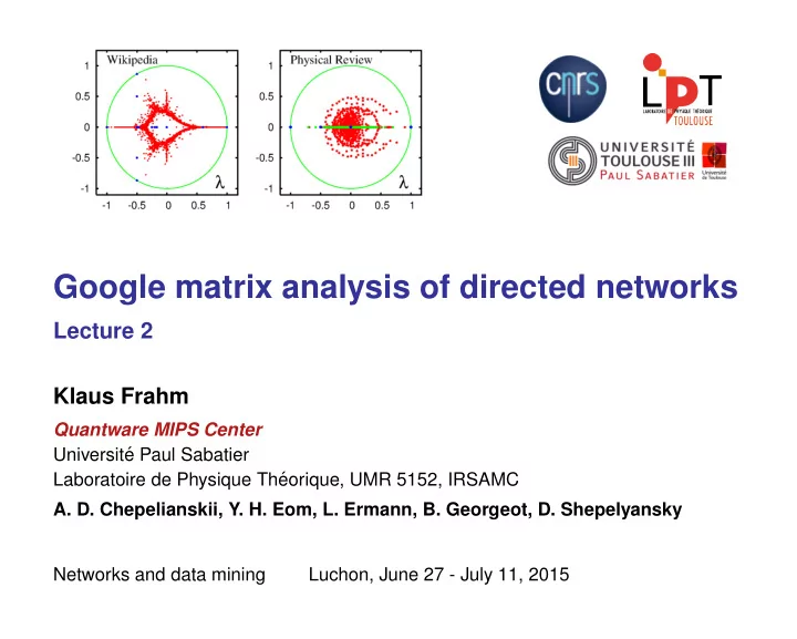
Spectrum of Wikipedia

Wikipedia 2009 : N = 3282257 nodes, Nℓ = 71012307 network links.

spectrum of S, Ns = 515 spectrum of S∗, Ns = 21198

nA = 6000 for both cases

3

Eigenvectors of Wikipedia

left (right): PageRank (CheiRank) black: PageRank (CheiRank) at α = 0.85 grey: PageRank (CheiRank) at α = 1 − 10−8 red and green: first two core space eigenvectors blue and pink: two eigenvectors with large imaginary part in the eigenvalue

4

Detail study of 200 selected eigenvectors with eigenvalues “close” to the unit circle: 5

Power law decay of eigenvectors:

|ψi(Ki)| ∼ Kb

i

for

Ki ≥ 104 ϕ = arg(λi)

6

Inverse participation ratio of eigenvectors:

ξIPR = (

j |ψi(j)|2)2/ j |ψi(j)|4

ϕ = arg(λi)

7

“Themes” of certain eigenvectors:

• 1
• 0.5

0.5 1 0.5

• 0.82
• 0.8
• 0.78
• 0.76
• 0.74
• 0.72

0.8 0.82 0.84 0.86 0.88 0.9 0.92 0.94 0.96 0.98 Australia

Switzerland

England Bangladesh New Zeland Poland Kuwait Iceland Austria Brazil China Australia Australia Canada England muscle-artery biology DNA RNA protein skin muscle-artery muscle-artery mathematics math (function, geometry,surface, logic-circuit) rail war

Gaafu Alif Atoll Quantum Leap

Texas-Dallas-Houston

Language music Bible poetry football song poetry aircraft

8

Chirikov Standard map

0.1 0.2 0.3 0.4 0.5 0.2 0.4 0.6 0.8 1 p x k=0.7 0.1 0.2 0.3 0.4 0.5 0.2 0.4 0.6 0.8 1 p x k=0.971635406

pn+1 = pn + k 2π sin(2π xn) xn+1 = xn + pn+1 x and p are taken modulo 1

and the symmetry

(x, p) → (1 − x, 1 − p)

allows to restrict:

x ∈ [0, 1] and p ∈ [0, 0.5].

Transition to “global” chaos at

kc = 0.971635406.

9

Perron-Frobenius matrix for chaotic maps

A new variant of the Ulam Method to construct the Perron-Frobenius matrix for the case of a mixed phase space:

• Subdivide x space in M cells and p space in M/2 cells with M

being an (even) integer number.

• Iterate (for a very long time: t ∼ 1011 − 1012) a classical trajectory

and attribute a new number to each new cell which is entered. At the same time count the number of transitions from cell i to cell j (⇒ nji).

• Calculate the N × N matrix

Gji = nji

• l nli
• f dimension N ≈ M 2/4 and which is a (sparse) Perron

Frobenius operator, i. e.: Gji ≥ 0,

j Gji = 1, Gji sparse.

10

M = 10, t = 106 ⇒ N = 35

0.1 0.2 0.3 0.4 0.5 0.2 0.4 0.6 0.8 1 p x 1 2 3 4 5 6

density plot of matrix elements

(blue=min=0, green=medium, red=max)

2 4 6 8 10 12 14 1 2 3 4 5 6

distribution of number of non-zero matrix elements per column

11

Eigenvalues

for M = 10, t = 106 and N = 35

• 1
• 0.5

0.5 1

• 1
• 0.5

0.5 1

λ

Phase space representation

• f

the eigenvector for λ0 = 1.

for M = 280, t = 1012 and N = 16609

• 1
• 0.5

0.5 1

• 1
• 0.5

0.5 1

λ

• 0.01

0.01 0.97 0.98 0.99 1

λ

12

Complex density of states

0.2 0.4 0.6 0.8 1 1.2 0.2 0.4 0.6 0.8 1 ρ(λ) |λ| M=280 M=200 M=140 M=100

13

Eigenvectors

λ0 = 1, M = 25, N = 177 λ0 = 1, M = 50, N = 641 λ0 = 1, M = 35, N = 332 λ0 = 1, M = 70, N = 1189

14

λ0 = 1 M = 140 N = 4417 λ0 = 1 M = 280 N = 16609

15

complex density of states:

0.1 0.2 0.3 0.6 0.8 1 ρ(λ) |λ| M=280 M=400 M=560 M=800 M=1120 M=1600

16

λ0 = 1, M = 1600, N = 494964, nA = 3000

17

λ1 = 0.99980431 M = 800 N = 127282 nA = 2000 λ2 = 0.99878108 M = 800 N = 127282 nA = 2000

18

Diffuson modes

0.01 0.02 0.03 5 10 15 20 γj j γ1 j2

γj = −2 ln(|λj|) γj ≈ γ1 j2

for j ≤ 5. What about eigenvectors for complex or real negative λj ? 19

λ6 = −0.49699831 +i 0.86089756 ≈ |λ6| ei 2π/3 M = 800 N = 127282 nA = 2000 λ19 = −0.71213331 +i 0.67961609 ≈ |λ19| ei 2π(3/8) M = 800 N = 127282 nA = 2000

20

λ8 = 0.00024596 +i 0.99239222 ≈ |λ8| ei 2π/4 M = 800 N = 127282 nA = 2000 λ13 = 0.30580631 +i 0.94120900 ≈ |λ13| ei 2π/5 M = 800 N = 127282 nA = 2000

21

Extrapolation of eigenvalues

γ1(M) in the limit M → ∞:

0.1 0.01 0.001 10-4 100 1000 γ1(M) M f(M) 2.36 M -1.30

f(M) = D M 1 + C

M

1 + B

M

D = 0.245 B = 13.1 C = 258 γ6(M) in the limit M → ∞:

0.01 0.1 1600 800 400 200 γ6(M) M 389 M -1.55

γ6(M) ≈ 389 M −1.55

for M ≥ 400. 22

Strong chaos

at k = 7, M = 140, t = 1011 and N = 9800

• 1
• 0.5

0.5 1

• 1
• 0.5

0.5 1

λ

0.1 0.2 0.3 0.005 0.01 γ1(M) M -1 d+e M -1 a (1+b M -1) c γclass.=0.0866

a ≈ 0.0857 ± 0.0036, d ≈ 0.0994 lim

M→∞ γ1(M) > 0

23

λ0 = 1 k = 7 M = 800 N = 319978 nA = 1500 λ1 = 0.93874817 k = 7 M = 800 N = 319978 nA = 1500

24

λ2 = −0.49264273 +i0.78912368 k = 7 M = 800 N = 319978 nA = 1500 λ8 = 0.87305253 k = 7 M = 800 N = 319978 nA = 1500

25

Separatrix map

¯ p = p + sin(2πx) ¯ x = x + Λ 2π ln(|¯ p|) (mod 1) Λ = Λc = 3.1819316

26

Phase space localization

27

References

• 1. D. L. Shepelyansky Fractal Weyl law for quantum fractal

eigenstates, Phys. Rev. E 77, p.015202(R) (2008).

• 2. L. Ermann and D. L. Shepelyansky, Ulam method and fractal

Weyl law for Perron-Frobenius operators, Eur. Phys. J. B 75, 299 (2010).

• 3. K. M. Frahm and D. L. Shepelyansky, Ulam method for the

Chirikov standard map, Eur. Phys. J. B 76, 57 (2010).

• 4. L. Ermann, K. M. Frahm and D. L. Shepelyansky, Spectral

properties of Google matrix of Wikipedia and other networks,

• Eur. Phys. J. B 86, 193 (2013).
• 5. K. M. Frahm and D. L. Shepelyansky, Poincar´

e recurrences and Ulam method for the Chirikov standard map, Eur. Phys. J. B 86, 322 (2013). 28