Goals Higher resolution Refinement Strategies for Single Particle - PDF document

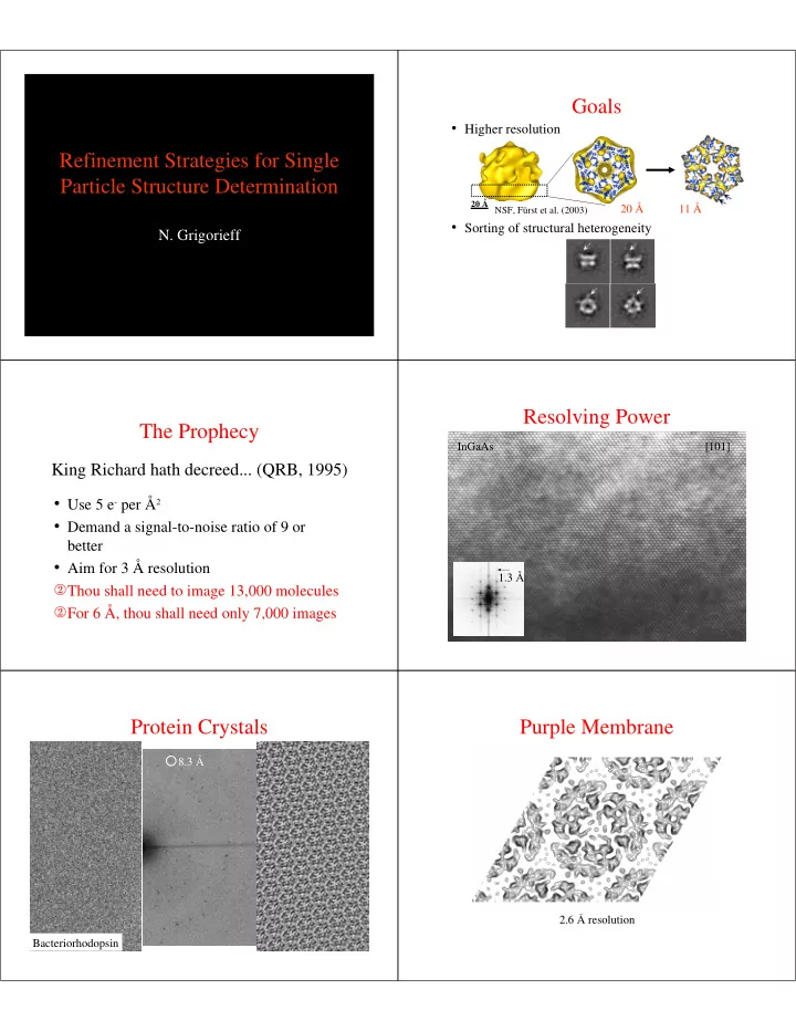
Goals • Higher resolution Refinement Strategies for Single Particle Structure Determination 20 Å 20 Å 11 Å NSF, Fürst et al. (2003) • Sorting of structural heterogeneity N. Grigorieff Resolving Power The Prophecy InGaAs [101] King Richard hath decreed... (QRB, 1995) • Use 5 e - per Å 2 • Demand a signal-to-noise ratio of 9 or better • Aim for 3 Å resolution 1.3 Å � Thou shall need to image 13,000 molecules � For 6 Å, thou shall need only 7,000 images Protein Crystals Purple Membrane 8.3 Å 2.6 Å resolution Bacteriorhodopsin

The Puzzle A Crazy Idea • Assume reliable resolution measure ������ ��� • Search entire parameter space for highest resolution • Given enough images, atomic resolution is reached 5 parameters • Example: to determine 3 angles, 1 deg step; two coordinates, 1 pixel step: 360 x 360 x 360 x 100 x 100 = 5 x 10 11 Additional parameters: 13000 particles: (5 x 10 11 ) 13000 structures to search CTF (3 parameters) Magnification • This is a big number! Beam Tilt (2 parameters) 200Å Refinement Strategy 1: Projection Matching Low-resolution structure Aligned Particles Reference Reference High-resolution structure (Expectation maximization) Strategy 2: Alignment in Strategy 3: MRA and Reciprocal Space Classification

Strategy 4: Maximum Likelihood ( ) ( ) ∫ φ φ Θ φ � � � � � � � � ∑ � + = � � � � � � �������������� ( ) � ∫ φ Θ φ � � � � ������������ � � � � = N = 4000 � � � SNR = 1/200 Maximum likelihood ( )   φ − �   � ( ) ( ) � � � alignment φ Θ =    −  φ Θ ����������� � � � ��� � � σ � π σ    �  �������� � �   φ ���������������������� X i � �� �������� N ������������� f Θ ������� ���������� σ ����������������� � � �������������������� Sigworth (1998), J. Struct. Biol. 122, 328-339 Sigworth (1998), J. Struct. Biol. 122, 328-339 Defocus/Astigmatism and ML processing of 2D crystals Magnification ��� ������������� Crystallography Alignment of individual unit cells using ML approach CTFFIND3 CTFTILT Problem 1: Local Optima Problem 2: Missing Views > 60º Particle Reference

Classification Using ML Problem 3: Heterogeneity ( ) ( ) ∫ φ φ Θ φ � � � � � � � � ∑ ∑∫ � � + = � � �������������� � � � � ( ) � ∑ ( ) Θ � φ Θ φ � � � � � � ������������ � = � � � � � � � � � ( )   φ −   � � ( ) � � ( ) � φ Θ =    −  φ Θ � � ����������� � � � ��� � � π σ σ �    �  � �������� �   • Misalignment of particles ( ) ( ) φ ∫ ����������� Θ = φ Θ � � � � � � • Lower resolution in disordered regions � � ���������� � • Loss of features φ ���������������������� X i � �� �������� N ������������� f Θ ������� ���������� σ ����������������� � � �������������������� Classification Using ML Problem 4: Processing Artifacts Low-resolution structure • Interpolation errors • Masking Aligned Particles Reference • Negative B-factor High-resolution • … structure SNR = 1/50 Difference N = 2000 map N = 1000, SNR = 1/20 Correlation alignment Problem 5: Noise Bias Seeing is NOT Always Believing ⊗ = 0 on average ⊗ > 0 align 100 Images 1000 Images Reference for 64x64 image: average correlation = 0.064

Resolution Measurement . Images of Particles Alignment Averaging FSC 100 Å Resolution Swiss Cheese Gedanken Experiments 1 0.9 0.8 Fourier Shell Correlation 0.7 0.6 0.5 0.4 9.2 Å 0.3 0.2 0.1 0 ∞ 20 10 6.7 Resolution [Å] N = 30000 Dangerous: SNR = 1/50 Boosting of high-resolution terms (application of a negative B-factor) Weighted Correlation Noise Bias Estimated resolution True resolution Alignment against 1 1 perfect reference ���� 0.8 0.8 �� (1 cycle only) �������� 0.6 0.6 Projection Test FSC FSC Model Reconstructions data 0.4 0.4 ���� (2 cubes) 0.2 0.2 �� �������� 0 0 0 0.1 0.2 0.3 0.4 0.5 0 0.1 0.2 0.3 0.4 0.5 Noise Resolution [pixel -1 ] Resolution [pixel -1 ] ∑ ( ) ∆Φ � � � � � � � � � [ ] ∈ = � � � � � � 1 ���� � � � � � ∑ ( ) � � � ��������� Noise � 0.8 [ ] ∈ ���� ���� � � � � � � ���� ��� only �� �� ( ) ( ) ∑ �������� �������� 0.6 † � � � � ��� FSC � � [ ] ��� = ∈ � � � � � � 0.4 �� � � � � � ��� ∑ ( ) ∑ ( ) Test Signal � � ���� � � � � 0.2 �� � � ��� data only [ ] [ ] ∈ ∈ �������� � � � � � � � � � � � � 0 � ) ∑ ( ) ( ∑ ( ) ( ) ( ) 0 0.1 0.2 0.3 0.4 0.5 � ��� ��� ��� ��� ��� � ��� ��� ��� ��� ��� � ��� ��� ��� ��� ��� = ≈ † � �� � � � �� � � � � � � �� � � � Correlation with perfect reference �� � Resolution [pixel -1 ] ����������������� � � � � � � [ ] ∈ � � � � � � �

Noise Reconstruction Coherence Constraint ) ∑ ( = � �� � � � �� � � � Linear Weighted Phase correlation correlation � � ���� ���� residual coefficient coefficient Reference ��� �� �� ��� �������� �������� ��� ��� ��� ��� ��� ��� ��� � � � ��� ��� ��� ��� ��� � ��� ��� ��� ��� ��� �� � ���������� ������ Acknowledgements • Ca Channel Matthias Wolf (Glossmann/Striessnig) • NSF/20S Johannes Fürst (Axel Brünger) • Noisy Face David DeRosier • Financial Support: HHMI, NIH, NSF