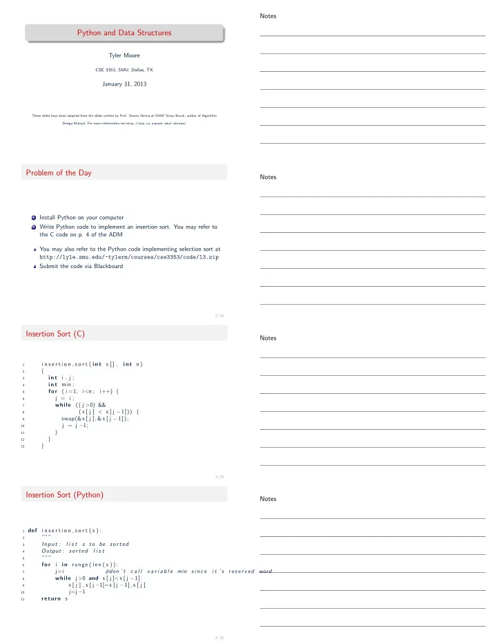
Python and Data Structures Tyler Moore CSE 3353, SMU, Dallas, TX - PDF document

Notes Python and Data Structures Tyler Moore CSE 3353, SMU, Dallas, TX January 31, 2013 These slides have been adapted from the slides written by Prof. Steven Skiena at SUNY Stony Brook, author of Algorithm Design Manual. For more information see http://www.cs.sunysb.edu/~skiena/ Problem of the Day Notes 1 Install Python on your computer 2 Write Python code to implement an insertion sort. You may refer to the C code on p. 4 of the ADM You may also refer to the Python code implementing selection sort at http://lyle.smu.edu/~tylerm/courses/cse3353/code/l3.zip Submit the code via Blackboard 2 / 32 Insertion Sort (C) Notes i n s e r t i o n s o r t ( int s [ ] , int n) 1 { 2 int i , j ; 3 min ; int 4 for ( i =1; i < n ; i++) { 5 j = i ; 6 (( j > 0) && while 7 ( s [ j ] < s [ j − 1])) { 8 swap(&s [ j ] ,& s [ j − 1]); 9 j = j − 1; 10 } 11 } 12 } 13 3 / 32 Insertion Sort (Python) Notes 1 def i n s e r t i o n s o r t ( s ) : ””” 2 Input : l i s t s to be s o r t e d 3 Output : s o r t e d l i s t 4 ””” 5 for i in range ( l e n ( s ) ) : 6 j=i #don ’ t c a l l v a r i a b l e min s i n c e i t ’ s r e s e r v e d word 7 while j > 0 and s [ j ] < s [ j − 1]: 8 s [ j ] , s [ j − 1]=s [ j − 1] , s [ j ] 9 j=j − 1 10 return s 11 4 / 32

Python Resources Notes Download from python.org for all major platforms I’ve written an online tutorial: http://lyle.smu.edu/~tylerm/courses/cse3353/python.html Beginning Python, Magnus Lie Hetland: http://link.springer. com/book/10.1007/978-1-4302-0634-7/page/1 5 / 32 Python Built-in Data Types Notes Recall that Python uses implicit, dynamic typing You can use casting functions float(), int() and str() to explicitly convert. In addition to numbers and strings, Python offers built-in support for lists, tuples, sets and dictionaries. 6 / 32 Working with lists Notes 1 > > s p o r t s =[ ’ f o o t b a l l ’ , ’ t e n n i s ’ , ’ i c e hockey ’ , ’ l a c r o s s e ’ , > ’ f i e l d hockey ’ , ’ b a s k e t b a l l ’ , ’ b a s e b a l l ’ , ’ swimming ’ ] 2 > > i n o r o u t =[ ’ out ’ , ’ both ’ , ’ i n ’ , ’ out ’ , ’ out ’ , ’ i n ’ , ’ out ’ , ’ i n ’ ] > 3 > > l e n ( s p o r t s ) #b u i l t − i n f u n c t i o n computes the l e n g t h of l i s t s > 4 8 5 > > s p o r t s l o c=z i p ( sports , i n o r o u t ) #b u i l t − i n element − wise > f u n c t i o n combines l i s t 6 > > s p o r t s l o c > 7 [ ( ’ f o o t b a l l ’ , ’ out ’ ) , ( ’ t e n n i s ’ , ’ both ’ ) , ( ’ i c e hockey ’ , ’ i n ’ ) , ( ’ l a c r o s s e ’ , ’ out ’ ) , ( ’ f i e l d hockey ’ , ’ out ’ ) , ( ’ b a s k e t b a l l ’ , ’ i n ’ ) , ( ’ b a s e b a l l ’ , ’ out ’ ) , ( ’ swimming ’ , ’ i n ’ ) ] 8 > > r a n d o m l i s t =[ ’ f o o t b a l l ’ , 3 , 6 . 7 , ’ham ’ ] #l i s t > elements don ’ t have to be the same type 7 / 32 List indexing Notes Python offers several ways to extract elements and sublists from a list. Syntactically you use square braces at the end of the list variable name, with the indices you want to access. Indices start at 0. You can get a range of values by including two numbers separated by a colon. If you use one number and a colon, it will give you the rest of the list. You can access the end of the list by using negative numbers 1 > > s p o r t s [ 2 ] > 2 ’ i c e hockey ’ 3 > > s p o r t s [ 1 : 3 ] > 4 [ ’ t e n n i s ’ , ’ i c e hockey ’ ] 5 > > > s p o r t s [ 2 : ] 6 [ ’ i c e hockey ’ , ’ l a c r o s s e ’ , ’ f i e l d hockey ’ , ’ b a s k e t b a l l ’ , ’ b a s e b a l l ’ , ’ swimming ’ ] 7 > > s p o r t s [ : 2 ] > 8 [ ’ f o o t b a l l ’ , ’ t e n n i s ’ ] 9 > > s p o r t s [ − 2] > 10 ’ b a s e b a l l ’ 11 > > s p o r t s [ − 2:] > 12 [ ’ b a s e b a l l ’ , ’ swimming ’ ] 8 / 32

Modifying a list Notes > bar = [ ’ b ’ , ’ a ’ , ’ j ’ , ’ h ’ , ’ l ’ ] > > > bar . append ( ’ o ’ ) > > > bar > > [ ’ b ’ , ’ a ’ , ’ j ’ , ’ h ’ , ’ l ’ , ’ o ’ ] > bar . pop ( ) > > ’ o ’ > bar > > [ ’ b ’ , ’ a ’ , ’ j ’ , ’ h ’ , ’ l ’ ] > bar . extend ( [ ’ y ’ , ’ x ’ ] ) > > > bar > > [ ’ b ’ , ’ a ’ , ’ j ’ , ’ h ’ , ’ l ’ , ’ y ’ , ’ x ’ ] > bar . i n s e r t ( ’w ’ ,3) > > Traceback ( most r e c e n t c a l l l a s t ) : F i l e ” < st di n > ” , l i n e 1 , i n < module > TypeError : an i n t e g e r i s r e q u i r e d > bar . i n s e r t (3 , ’w ’ ) > > > bar > > [ ’ b ’ , ’ a ’ , ’ j ’ , ’w ’ , ’ h ’ , ’ l ’ , ’ y ’ , ’ x ’ ] > bar . s o r t () > > > bar > > [ ’ a ’ , ’ b ’ , ’ h ’ , ’ j ’ , ’ l ’ , ’w ’ , ’ x ’ , ’ y ’ ] > bar [ : : − 1 ] > > [ ’ y ’ , ’ x ’ , ’w ’ , ’ l ’ , ’ j ’ , ’ h ’ , ’ b ’ , ’ a ’ ] 9 / 32 Tuples and sets Notes Tuples are immutable lists Sets are unordered lists > t = (4 ,6 ,2 ,3) > > > t [0]=5 > > Traceback ( most r e c e n t c a l l l a s t ) : F i l e ” < st di n > ” , l i n e 1 , i n < module > TypeError : ’ t u p l e ’ o b j e c t does support item assignment not > s = { 3 ,9 ,6 ,2 } > > > s [ 2 ] > > Traceback ( most r e c e n t c a l l l a s t ) : F i l e ” < st di n > ” , l i n e 1 , i n < module > TypeError : ’ s e t ’ o b j e c t does support i n d e x i n g not > 6 i n s > > True > 7 s > > i n F a l s e 10 / 32 Dictionaries Notes Dictionaries map keys to values. Both the keys and values can be of any type, from strings to numbers, to other dictionaries. 1 > > from sampledata import ∗ > 2 > > uni > 3 { ’ Jones ’ : ’ Oxford ’ , ’ G i l l i a m ’ : ’ O c c i d e n t a l ’ , ’ C l e e s e ’ : ’ Cambridge ’ , ’Chapman ’ : ’ Cambridge ’ , ’ I d l e ’ : ’ Cambridge ’ , ’ P a l i n ’ : ’ Oxford ’ } 4 > > uni [ ’ P a l i n ’ ] > 5 ’ Oxford ’ 6 > > uni [ ’ P a l i n ’ ] = ’ Oxford U n i v e r s i t y ’ > 7 > > uni [ ’ P a l i n ’ ] > 8 ’ Oxford U n i v e r s i t y ’ 9 > > uni . keys ( ) > 10 [ ’ Jones ’ , ’ G i l l i a m ’ , ’ C l e e s e ’ , ’Chapman ’ , ’ I d l e ’ , ’ P a l i n ’ ] 11 / 32 Dictionaries Notes You can also start from an empty dictionary and then add values: s p o r t 2 t y p e = {} s p o r t 2 t y p e [ ’ f o o t b a l l ’ ]= ’ out ’ s p o r t 2 t y p e [ ’ i c e hockey ’ ]= ’ i n ’ > s p o r t 2 t y p e > > { ’ i c e hockey ’ : ’ i n ’ , ’ f o o t b a l l ’ : ’ out ’ } 12 / 32