Getting to Know grid Graphics Paul Murrell, The University of - - PDF document

23/11/2017 Getting to Know grid Graphics file:///home/pmur002/fosFiles/Courses/NZSA2017/Slides/grid-slides.html 1/44

Getting to Know grid Graphics

Paul Murrell, The University of Auckland, December 2017 An overview of the short course

Getting to Know grid Graphics Introduction

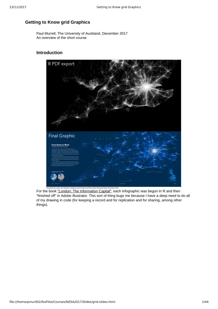
For the book "London: The Information Capital", each infographic was begun in R and then "finished off" in Adobe Illustrator. This sort of thing bugs me because I have a deep need to do all

• f my drawing in code (for keeping a record and for replication and for sharing, among other

things).

23/11/2017 Getting to Know grid Graphics file:///home/pmur002/fosFiles/Courses/NZSA2017/Slides/grid-slides.html 2/44

Introduction

One of the distinguishing features of the R graphics system, and the 'grid' graphics system in particular, is that it allows you fine control over details, including access to more advanced graphical features and details. As a "dramatic" demonstration of this idea, the image on this slide was generated completely in R. This course will try to reveal how 'grid' works so that you can do this sort of thing yourself.

Where is grid ?

grDevices grid graphics lattice ggplot2 ... plotrix maps ... SVG PNG PDF

The 'grid' package provides an ALTERNATIVE graphics system to the 'graphics' package ("base" graphics). Many packages define plotting functions based on 'graphics', but there are some important ones based on 'grid', such as 'lattice' and 'ggplot2'.

23/11/2017 Getting to Know grid Graphics file:///home/pmur002/fosFiles/Courses/NZSA2017/Slides/grid-slides.html 3/44

Where is grid ?

library(lattice) xyplot(mpg ~ disp, mtcars)

When you draw a plot with 'lattice' or 'ggplot2', the actual drawing is being done by 'grid'.

Exploring grid Grobs

library(grid) grid.ls() plot_01.background plot_01.xlab plot_01.ylab plot_01.ticks.top.panel.1.1 plot_01.ticks.left.panel.1.1 plot_01.ticklabels.left.panel.1.1 plot_01.ticks.bottom.panel.1.1 plot_01.ticklabels.bottom.panel.1.1 plot_01.ticks.right.panel.1.1 plot_01.xyplot.points.panel.1.1 plot_01.border.panel.1.1

When you draw something with 'grid', a record is kept of the objects that are drawn. 'grid' calls these objects "grobs" (graphical objects). The grid.ls() function can be used to list the grobs on the current page.

Exploring grid Grobs

Some other functions that help with exploring grobs:

grid.grep(path) Search for a grob that matches 'path'. showGrob(gPath) Highlight grob that matches 'gPath'. grobBrowser()

SVG version with grob names as tooltips (from the 'gridDebug' package).

23/11/2017 Getting to Know grid Graphics file:///home/pmur002/fosFiles/Courses/NZSA2017/Slides/grid-slides.html 4/44

grid Viewports

xyplot(mpg ~ disp, mtcars)

When you draw something with 'grid', a record is also kept of any "viewports" that were created. A viewport is a rectangular sub-region on the page.

Exploring grid Viewports

grid.ls(viewports=TRUE, grobs=FALSE) ROOT plot_01.toplevel.vp plot_01.xlab.vp plot_01.ylab.vp plot_01.figure.vp plot_01.panel.1.1.vp plot_01.strip.1.1.off.vp plot_01.strip.left.1.1.off.vp plot_01.panel.1.1.off.vp

The grid.ls() function can also be used to list the viewports on the current page. (The output on this slide has been trimmed and tidied to fit on one slide.)

Exploring grid Viewports

grid.ls(viewports=TRUE, fullNames=TRUE) viewport[ROOT] rect[plot_01.background] viewport[plot_01.toplevel.vp] viewport[plot_01.xlab.vp] text[plot_01.xlab] upViewport[1] viewport[plot_01.ylab.vp] text[plot_01.ylab] upViewport[1] viewport[plot_01.figure.vp]

This is the first few lines of the complete output from grid.ls() that shows both viewports and grobs (and therefore the nesting of grobs within viewports).

23/11/2017 Getting to Know grid Graphics file:///home/pmur002/fosFiles/Courses/NZSA2017/Slides/grid-slides.html 5/44

Exploring grid Viewports

Some other functions that help with exploring viewports:

showViewport(vp)

Highlight viewport that matches 'vp'.

current.viewport()Returns the current viewport.

Ideally, a package will document the naming scheme that it uses for grobs and viewports. Ideally, a package will have a naming scheme!

Exercise

The purpose of this exercise is to make use of the grid.ls() function. The following code creates a 'lattice' scatterplot:

library(lattice) xyplot(mpg ~ disp, mtcars, main="Fast Cars")

• 1. What is the name of the grob that represents the main title on the scatterplot?
• 2. What is the name of the viewport that the main title is drawn within?

Why Grobs ?

library(lattice) barchart(Party ~ Amount_Donated, sortedTotals)

Total Donated

United Future Independent Green Party Democrats for Social Credit Focus New Zealand New Zealand First Party ACT New Zealand Conservative MANA Movement Māori Party Internet Party Labour Party National Party 500000 1000000

One benefit of having access to the low-level 'grid' grobs is that we can make detailed customisations to a plot that was drawn with a high-level function where the high-level function does not provide control over enough of the details. In this case, I want to remove the border around the lattice panel.

Why Grobs ?

library(grid) grid.ls() plot_01.background plot_01.xlab plot_01.ticks.top.panel.1.1 plot_01.ticklabels.left.panel.1.1 plot_01.ticks.bottom.panel.1.1 plot_01.ticklabels.bottom.panel.1.1 plot_01.abline.v.panel.1.1 plot_01.barchart.abline.v.panel.1.1 plot_01.barchart.rect.panel.1.1 plot_01.border.panel.1.1

If I can find out what the grob is called ...

23/11/2017 Getting to Know grid Graphics file:///home/pmur002/fosFiles/Courses/NZSA2017/Slides/grid-slides.html 6/44

Why Grobs ?

library(grid) grid.remove("plot_01.border.panel.1.1")

Total Donated

United Future Independent Green Party Democrats for Social Credit Focus New Zealand New Zealand First Party ACT New Zealand Conservative MANA Movement Māori Party Internet Party Labour Party National Party 500000 1000000

... then I can remove it with grid.remove().

Working With Grobs

Functions that can be used to access grobs:

grid.remove()Remove a grob. grid.edit()

Modify a grob component.

grid.get()

Get a copy of a grob component.

grid.set()

Replace a grob component. Each function takes the name of a grob as its first argument. The name argument can be a regular expression, if you specify 'grep=TRUE'. You can work with more than one grob at once if you specify 'global=TRUE'.

Modifying Grobs

library(grid) t <- grid.get("plot_01.ticklabels.bottom.panel.1.1") names(t) [1] "label" "x" "y" "just" [5] "hjust" "vjust" "rot" "check.overlap" [9] "name" "gp" "vp" t$just [1] "centre" "top"

Grobs are just lists with components.

23/11/2017 Getting to Know grid Graphics file:///home/pmur002/fosFiles/Courses/NZSA2017/Slides/grid-slides.html 7/44

Modifying Grobs

library(grid) grid.edit("plot_01.ticklabels.bottom.panel.1.1", just=c("left", "top"))

Total Donated

United Future Independent Green Party Democrats for Social Credit Focus New Zealand New Zealand First Party ACT New Zealand Conservative MANA Movement Māori Party Internet Party Labour Party National Party 500000 1000000

We can use grid.edit() to change the value of a component. However, we may NOT edit 'name' or 'vp' components of a grob.

Modifying Grobs

library(grid) gpar(col="blue", lwd=3, lty="dashed") $col [1] "blue" $lwd [1] 3 $lty [1] "dashed"

The value of the 'gp' component of a grob is created with the gpar() function.

Modifying Grobs

Common gpar() settings:

col (border) colour. fill fill colour. lty line type. lwd line width. cex text size multiplier.

The other gpar() settings:

fontsize

The size of text (in points).

lineheight Vertical height of a line of text (multiplier). For vertical positioning of multi-line text. fontface

"plain", "bold", "italic", or "bolditalic".

fontfamily "sans", "serif", "mono", or the name of a font family that makes sense on the current

graphics device.

lineend

"round", "square", or "butt". The shape used at the end of lines.

linejoin

"round", "mitre", "bevel". The shape used at line corners.

linemitre Number used to decide when mitre joins become bevel joins. lex

Line expansion multiplier (affects line width).

23/11/2017 Getting to Know grid Graphics file:///home/pmur002/fosFiles/Courses/NZSA2017/Slides/grid-slides.html 8/44

Modifying Grobs

library(grid) grid.edit("plot_01.ticklabels.bottom.panel.1.1", gp=gpar(col="grey"))

Total Donated

United Future Independent Green Party Democrats for Social Credit Focus New Zealand New Zealand First Party ACT New Zealand Conservative MANA Movement Māori Party Internet Party Labour Party National Party 500000 1000000

Modifying the 'gp' component of a grob ONLY changes the gpar() settings that are given new values.

Exercise

The purpose of this exercise is to make use of the grid.edit() and grid.remove() functions. The following code creates a 'lattice' scatterplot:

library(lattice) xyplot(mpg ~ disp, mtcars, main="Fast Cars")

• 1. Change the colour of the main title to red.
• 2. Remove the main title from the plot.

Exercise

This is the result you are looking for (before you remove the title):

23/11/2017 Getting to Know grid Graphics file:///home/pmur002/fosFiles/Courses/NZSA2017/Slides/grid-slides.html 9/44

Why Viewports ?

Credit: John G. Bullock, Yale University.

John Bullock made use of the 'lattice' viewports that were created in this multi-panel plot to centre the text below each row of plots. (He did not use the 'xlab' argument to xyplot() because he wanted greater control over the vertical placement of the text.)

Why Viewports ?

Credit: John G. Bullock, Yale University.

John could do this because it is possible to revisit the viewports that are created when a plot is drawn with 'grid'.

23/11/2017 Getting to Know grid Graphics file:///home/pmur002/fosFiles/Courses/NZSA2017/Slides/grid-slides.html 10/44

Navigating Viewports

xyplot(mpg ~ disp, mtcars)

When you draw something with 'grid', a record is kept of any "viewports" that were created. A viewport is a rectangular sub-region on the page.

Navigating Viewports

grid.ls(viewports=TRUE, fullNames=TRUE) viewport[ROOT] rect[plot_01.background] viewport[plot_01.toplevel.vp] viewport[plot_01.xlab.vp] text[plot_01.xlab] upViewport[1] viewport[plot_01.ylab.vp] text[plot_01.ylab] upViewport[1] viewport[plot_01.figure.vp]

Viewports can be nested within each other.

23/11/2017 Getting to Know grid Graphics file:///home/pmur002/fosFiles/Courses/NZSA2017/Slides/grid-slides.html 11/44

Navigating Viewports

Viewports can be nested within each other.

Navigating Viewports

downViewport("plot_01.toplevel.vp") grid.rect(gp=gpar(col=NA, fill=rgb(0,1,0,.5)))

It is possible to revisit the viewports that a plot has created with the downViewport() function (and the name of the viewport we want to visit).

23/11/2017 Getting to Know grid Graphics file:///home/pmur002/fosFiles/Courses/NZSA2017/Slides/grid-slides.html 12/44

Navigating Viewports

downViewport("plot_01.panel.1.1.vp") grid.rect(gp=gpar(col=NA, fill=rgb(1,0,0,.5)))

It is possible to revisit the viewports that a plot has created with the downViewport() function (and the name of the viewport we want to visit). NOTE that drawing occurs relative to the viewport that we are currently in (by default, grid.rect() fills the entire viewport).

Navigating Viewports

upViewport() grid.rect(gp=gpar(col=NA, fill=rgb(0,0,1,.5)))

We can navigate up the viewport tree as well, using the upViewport() function.

23/11/2017 Getting to Know grid Graphics file:///home/pmur002/fosFiles/Courses/NZSA2017/Slides/grid-slides.html 13/44

Exercise

The purpose of this exercise is to make use of the downViewport() function. The following code creates a 'lattice' scatterplot:

library(lattice) xyplot(mpg ~ disp, mtcars, main="Fast Cars")

• 1. Navigate to the viewport that the main title was drawn in and draw a rectangle to show that you

are in the right place.

Exercise

This is the result you are looking for:

23/11/2017 Getting to Know grid Graphics file:///home/pmur002/fosFiles/Courses/NZSA2017/Slides/grid-slides.html 14/44

Why Viewports ?

Credit: Pascal A. Niklaus, University of Zurich.

Pascal Niklaus wanted to add letter labels in the top-left corner of each of his plots.

Why Viewports ?

Credit: Pascal A. Niklaus, University of Zurich.

These letter labels are difficult to position using the coordinate system provided by the scales on the plot axes.

23/11/2017 Getting to Know grid Graphics file:///home/pmur002/fosFiles/Courses/NZSA2017/Slides/grid-slides.html 15/44

Why Viewports ?

Credit: Brad Boehmke.

Here is a similar example, with more elaborate text annotations, this time on a 'ggplot2' plot.

Viewport Coordinates

xyplot(mpg ~ disp, mtcars) downViewport("plot_01.panel.1.1.vp")

Every 'grid' viewport has several coordinate systems associated with it.

23/11/2017 Getting to Know grid Graphics file:///home/pmur002/fosFiles/Courses/NZSA2017/Slides/grid-slides.html 16/44

Viewport Coordinates

grid.text("native", x=unit(300, "native"), y=unit(30, "native"), just=c("left", "bottom"))

The unit() function associates a value with a coordinate system. "Native" coordinates are relative to the 'xscale' and 'yscale' on the viewport.

Viewport Coordinates

grid.text("absolute", x=unit(1, "in"), y=unit(1, "cm"), just=c("left", "bottom"))

Absolute coordinates include "in", "cm", and "pt". All are measured from the bottom-left corner of the viewport.

23/11/2017 Getting to Know grid Graphics file:///home/pmur002/fosFiles/Courses/NZSA2017/Slides/grid-slides.html 17/44

Viewport Coordinates

grid.text("normalised", x=unit(.75, "npc"), y=unit(.5, "npc"), just=c("left", "bottom"))

Normalised ("npc") coordinates are 0-to-1 along each side of the viewport.

Viewport Coordinates

grid.text("normalised - absolute", x=unit(1, "npc") - unit(1, "cm"), y=unit(1, "npc") - unit(1, "cm"), just=c("right", "top"))

We can use simple arithmetic on units. In this case, we are positioning text a fixed amount in from the top-right corner of a viewport.

23/11/2017 Getting to Know grid Graphics file:///home/pmur002/fosFiles/Courses/NZSA2017/Slides/grid-slides.html 18/44

Drawing Grobs

Some basic shapes that 'grid' can draw:

grid.rect(x,y,w,h)

rectangles.

grid.circle(x,y,r)

circles.

grid.lines(x,y)

straight lines through (x,y).

grid.segments(x0,y0,x1,y1) straight lines from (x0,y0) to (x1,y1). grid.text(label,x,y)

text. The other "shapes" that 'grid' can draw:

grid.move.to(x,y)

set current "pen" location.

grid.line.to(x,y)

straight line from "pen" location to (x,y) (and set "pen" location to (x,y)).

grid.polyline(x,y,id)

straight lines through multiple sets of (x,y).

grid.xspline(x,y,shape)

smooth curve relative to (x,y) control points.

grid.roundrect(x,y,w,h,r) rectangle with rounded corners. grid.polygon(x,y)

polygon defined by (x,y) (automatically closing last point to first point).

grid.path(x,y,id)

path (potentially defined by multiple polygons).

grid.raster(image,x,y,w,h) raster image. grid.curve(x1,y1,x2,y2)

smooth curve between two end points.

grid.points(x,y,pch)

data symbols at (x,y) (default coordinate system is "native"!).

Drawing Grobs

grid.rect(x=unit(.2, "npc"), y=unit(100, "native"), width=unit(1, "in"), height=unit(1, "lines"))

Whenever we draw a grob, we can specify the position and size of the grob using any of the available coordinate systems (the default is almost always "npc").

23/11/2017 Getting to Know grid Graphics file:///home/pmur002/fosFiles/Courses/NZSA2017/Slides/grid-slides.html 19/44

Drawing Grobs

grid.circle(x=1:5/6, y=.5, r=1:5/25)

For most grobs, the location and size specifications can be vectors so that a single call to a 'grid' function can produce multiple shapes.

Exercise

The purpose of this exercise is to make use of the unit() function as well as 'grid' functions that draw basic shapes. The following code creates a 'lattice' scatterplot:

library(lattice) xyplot(mpg ~ disp, mtcars, main="Fast Cars")

• 1. Navigate to the viewport that the data symbols were drawn in and draw a horizontal line at mpg

== 25.

• 2. Draw a label just above and to the right of the symbol for the "Pontiac Firebird" (disp=400,

mpg=19.2).

23/11/2017 Getting to Know grid Graphics file:///home/pmur002/fosFiles/Courses/NZSA2017/Slides/grid-slides.html 20/44

Exercise

This is the result you are looking for:

Why Viewports ?

Credit: Tom Wright, affiliation unknown.

Tom Wright has a 'lattice' plot with too many empty panels.

23/11/2017 Getting to Know grid Graphics file:///home/pmur002/fosFiles/Courses/NZSA2017/Slides/grid-slides.html 21/44

Why Viewports ?

We can do a little bit better if we draw separate 'lattice' plots in separate 'grid' viewports.

Why Viewports ?

This version of the "improved" plot has the 'grid' viewports highlighted by coloured rectangles.

23/11/2017 Getting to Know grid Graphics file:///home/pmur002/fosFiles/Courses/NZSA2017/Slides/grid-slides.html 22/44

Starting a New Page

grid.newpage()

With raw 'grid', we have to explicitly call the grid.newpage() function to start a new page/screen. All other 'grid' functions just add to the current page/screen. 'lattice' plotting functions, like xyplot(), automatically start a new page, unless you tell them not to with something like print(xyplot(...), newpage=FALSE).

23/11/2017 Getting to Know grid Graphics file:///home/pmur002/fosFiles/Courses/NZSA2017/Slides/grid-slides.html 23/44

Creating Viewports

vp <- viewport(width=.5, height=.5) pushViewport(vp) grid.rect(gp=gpar(col=NA, fill="grey80"))

We can create a new viewport description with the viewport() function. In this case, we are describing a viewport that is half the width of the page and half the height of the page (the default is to be centred on the middle of the page). The location and size of viewports are specified using the unit() function, just like for grobs (and the default coordinate system is "npc"). We create a viewport on the page using the pushViewport() function. After the "push", all drawing

• ccurs within that viewport. In this case, we draw a rectangle that shows the extent of the

viewport that we have created.

23/11/2017 Getting to Know grid Graphics file:///home/pmur002/fosFiles/Courses/NZSA2017/Slides/grid-slides.html 24/44

Creating Viewports

vp2 <- viewport(x=0, y=.5, width=.5, height=.5, just=c("left", "bottom")) pushViewport(vp2) grid.rect()

When we push a viewport, the viewport description is always relative to the current viewport. In this case, we define and push a viewport that is in the top-left quarter of the current viewport. We draw a rectangle to show the extent of this new viewport.

23/11/2017 Getting to Know grid Graphics file:///home/pmur002/fosFiles/Courses/NZSA2017/Slides/grid-slides.html 25/44

Creating Viewports

grid.newpage() pushViewport(vp) print(xyplot(mpg ~ disp, mtcars), newpage=FALSE)

A 'lattice' plot is just a lot of pushing viewports and drawing shapes. We can tell a 'lattice' plot to do its pushing of viewports and drawing of shapes in the current viewport rather than starting a new page all for itself. We do this by explicitly calling print() on the plot and setting the 'newpage' argument to FALSE.

Exercise

The purpose of this exercise is to make use of the viewport() and pushViewport() functions. The following code creates a 'lattice' scatterplot:

library(lattice) xyplot(mpg ~ disp, mtcars, main="Fast Cars")

• 1. Create a viewport in the bottom-right quarter of the page and draw the plot in that viewport.

23/11/2017 Getting to Know grid Graphics file:///home/pmur002/fosFiles/Courses/NZSA2017/Slides/grid-slides.html 26/44

Exercise

This is the result you are looking for:

Summary

'lattice' plots create 'grid' grobs and viewports. grid.ls() lists grobs and viewports. grid.remove() and grid.edit() modify grobs. downViewport() and upViewport() navigate between viewports. grid.rect(), grid.text(), etc draw new grobs. gpar() controls graphical parameters. viewport() and pushViewport() create new viewports. 'lattice' plots can be drawn within any viewport. Nuff said

23/11/2017 Getting to Know grid Graphics file:///home/pmur002/fosFiles/Courses/NZSA2017/Slides/grid-slides.html 27/44

Where is grid ?

library(ggplot2) qplot(disp, mpg, data=mtcars, main="Fast Cars")

When you draw a plot with 'lattice' or 'ggplot2', the actual drawing is being done by 'grid'.

Exploring grid Grobs

grid.ls() layout

One difference between the grobs created by 'lattice' and the grobs created by 'ggplot2' is that the latter produces a single grob that draws everything. To see all of the individual grobs that are drawn, we need the grid.force() function.

Exploring grid Grobs

grid.force() grid.ls() layout background.1-7-10-1 panel.6-4-6-4 grill.gTree.537 panel.background..rect.528 panel.grid.minor.y..polyline.530 panel.grid.minor.x..polyline.532 panel.grid.major.y..polyline.534 panel.grid.major.x..polyline.536 NULL geom_point.points.524

Another difference between the grobs created by 'lattice' and the grobs created by 'ggplot2' is that the latter are arranged in a hierarchy. For example, there is a "panel" grob, with a "grill" as its child, and various rectangles and polylines as children of that. Yet another difference is that the 'ggplot2' naming scheme is less intuitive and less complete (and undocumented).

23/11/2017 Getting to Know grid Graphics file:///home/pmur002/fosFiles/Courses/NZSA2017/Slides/grid-slides.html 28/44

Modifying Grobs

grid.edit("title::text", grep=TRUE, gp=gpar(col="red"))

10 15 20 25 30 35 100 200 300 400

disp mpg

Fast Cars

We can use grid.edit() to change the value of a component just like with 'lattice' plots. There are two extra complications here: first, we are using 'grep=TRUE' to use grob name pattern matching; second, we are using a grob name *path* to specify a grob with "text" in its name that is the child of a grob with "title" in its name.

Modifying Grobs

grid.remove("title.2-4-2-4")

10 15 20 25 30 35 100 200 300 400

disp mpg

We can use grid.remove() to remove grobs just like with 'lattice' plots. Notice that removing a parent grob also removes its children.

23/11/2017 Getting to Know grid Graphics file:///home/pmur002/fosFiles/Courses/NZSA2017/Slides/grid-slides.html 29/44

Navigating Viewports

qplot(disp, mpg, data=mtcars, main="Fast Cars") grid.force() grid.ls(viewports=TRUE, fullNames=TRUE) viewport[ROOT] viewport[layout] forcedgrob[layout] viewport[background.1-7-10-1] forcedgrob[background.1-7-10-1] upViewport[1] viewport[panel.6-4-6-4] forcedgrob[panel.6-4-6-4] gTree[grill.gTree.659] rect[panel.background..rect.650]

'ggplot2' creates viewports just like 'lattice'.

Navigating Viewports

downViewport("panel.3-4-3-4") grid.rect(gp=gpar(col=NA, fill=rgb(0,1,0,.5)))

It is possible to revisit the viewports that 'ggplot2' has created, just like with 'lattice'. However, one difference is that the viewport representing the 'ggplot2' plot region does NOT have a "native" scale corresponding to the axis scales.

Exercise

The purpose of this exercise is to make use of 'grid' functions with a 'ggplot2' plot. The following code creates a 'ggplot2' scatterplot:

library(ggplot2) qplot(disp, mpg, data=mtcars, main="Fast Cars")

• 1. Navigate to the viewport that the main title was drawn in and draw a rectangle to show the

extent of the viewport.

• 2. Edit the title grob to move it to the right-hand edge of the plot.
• 3. Remove the rectangle that you just drew.

23/11/2017 Getting to Know grid Graphics file:///home/pmur002/fosFiles/Courses/NZSA2017/Slides/grid-slides.html 30/44

Exercise

This is the result you are looking for:

Where is grid ?

library(vcd) mosaic(Titanic)

A number of other packages build on top of 'grid' (or 'lattice' or 'ggplot2'), but there is no guarantee of a naming scheme for grobs and viewports.

23/11/2017 Getting to Know grid Graphics file:///home/pmur002/fosFiles/Courses/NZSA2017/Slides/grid-slides.html 31/44

Exploring grid Grobs

grid.ls() GRID.lines.822 GRID.lines.823 disc:Class=1st,Sex=Male,Age=Child,Survived=No, circle:Class=1st,Sex=Male,Age=Child,Survived=No, rect:Class=1st,Sex=Male,Age=Child,Survived=Yes rect:Class=1st,Sex=Male,Age=Adult,Survived=No rect:Class=1st,Sex=Male,Age=Adult,Survived=Yes GRID.lines.824 GRID.lines.825 disc:Class=1st,Sex=Female,Age=Child,Survived=No,

Where is grid ?

grDevices grid graphics lattice ggplot2 ... plotrix maps ... SVG PNG PDF gridGraphics gridSVG

The 'gridGraphics' package provides a way to convert plots drawn with the 'graphics' package into identical plots drawn with 'grid'.

23/11/2017 Getting to Know grid Graphics file:///home/pmur002/fosFiles/Courses/NZSA2017/Slides/grid-slides.html 32/44

Where is grid ?

plot(mpg ~ disp, mtcars, pch=16, main="Fast Cars") library(gridGraphics) grid.echo()

We can draw a plot based on 'graphics' then call grid.echo() to convert it into 'grid' grobs and viewports.

Exploring grid Grobs

grid.ls() graphics-background graphics-plot-1-points-1 graphics-plot-1-bottom-axis-line-1 graphics-plot-1-bottom-axis-ticks-1 graphics-plot-1-bottom-axis-labels-1 graphics-plot-1-left-axis-line-1 graphics-plot-1-left-axis-ticks-1 graphics-plot-1-left-axis-labels-1 graphics-plot-1-box-1 graphics-plot-1-main-1 graphics-plot-1-xlab-1 graphics-plot-1-ylab-1

Navigating Viewports

grid.ls(viewports=TRUE, fullNames=TRUE) viewport[ROOT] rect[graphics-background] viewport[graphics-root] upViewport[1] downViewport[graphics-root] viewport[graphics-inner] upViewport[2] downViewport[graphics-root] downViewport[graphics-inner] viewport[graphics-figure-1]

23/11/2017 Getting to Know grid Graphics file:///home/pmur002/fosFiles/Courses/NZSA2017/Slides/grid-slides.html 33/44

Exercise

The purpose of this exercise is to make use of 'grid' functions with a 'graphics' plot. The following code creates a 'graphics' scatterplot:

plot(mpg ~ disp, mtcars, pch=16, main="Fast Cars")

• 1. Convert the plot to an identical 'grid' plot, change the title to red.
• 2. Remove the title.

Exercise

This is the result you are looking for (before you delete the title):

23/11/2017 Getting to Know grid Graphics file:///home/pmur002/fosFiles/Courses/NZSA2017/Slides/grid-slides.html 34/44

Why grid ?

The concepts of viewports in the 'grid' package provide a better basis (than the 'graphics' package) for producing complex plots like 'lattice' multi-panel conditioning plots. For example, how does 'lattice' leave enough space for the axis labels and the plot legend, but make the panels as large as possible ?

Why grid ?

Plots produced by 'ggplot2' also benefit from 'grid' concepts like viewports to determine the arrangement of pieces of a complex plot within a page.

23/11/2017 Getting to Know grid Graphics file:///home/pmur002/fosFiles/Courses/NZSA2017/Slides/grid-slides.html 35/44

Why grid ?

The fact that 'grid' is a general-purpose graphics system (not just for plots) means that 'grid' concepts like viewports can be applied to things like arranging photos together on a page.

Why grid ?

The fact that 'grid' is a general-purpose graphics system also means that 'grid' can be used as a rudimentary desktop publishing system (code-based, of course).

23/11/2017 Getting to Know grid Graphics file:///home/pmur002/fosFiles/Courses/NZSA2017/Slides/grid-slides.html 36/44

grid Layouts

The approach that 'lattice' takes is to use a 'grid' "layout". A layout divides up a (parent) viewport into a number of rows and columns and subsequent (child) viewports that are pushed beneath the (parent) viewport with the layout can occupy a subset of the cells in the (parent) layout.

Creating Layouts

widths <- unit(c(1, 2, 1), c("null", "null", "cm")) lay <- grid.layout(3, 3, widths=widths) vplay <- viewport(layout=lay) pushViewport(vplay) pushViewport(viewport(layout.pos.row=2, layout.pos.col=2)) grid.rect(gp=gpar(col=NA, fill=rgb(1,0,0,.5)))

A layout can be specified as part of the description of a viewport. A viewport can specify its location in terms of the rows and columns of a parent layout.

23/11/2017 Getting to Know grid Graphics file:///home/pmur002/fosFiles/Courses/NZSA2017/Slides/grid-slides.html 37/44

Exercise

The purpose of this exercise is to make use of the grid.layout() function.

• 1. Produce a layout like the diagram below.

+-----------------------------------------+ | w=7/9 5 h=0.5/5.5 | +-----+-----------------------------+-----+ | | 1 h=1.0/5.5 | | | +-----------------------------+ | | 6 | 2 h=1.0/5.5 | 7 | | +-----------------------------+ | |w=1/9| 3 h=1.0/5.5 |w=1/9| | +-----------------------------+ | | | | | | | 4 h=2.0/5.5 | | | | | | +-----+-----------------------------+-----+

Credit: Julio Sergio Santana.

Exercise

This is the result you are looking for (the grid.show.layout() function takes a 'grid' layout as its argument and draw a diagram of the layout):

23/11/2017 Getting to Know grid Graphics file:///home/pmur002/fosFiles/Courses/NZSA2017/Slides/grid-slides.html 38/44

Viewport Coordinates

grid.rect(width=stringWidth("axis label"))

The stringWidth() function lets us specify a width in terms of the size of a piece of text (like a label

• n a plot axis).

There is also a stringHeight() function. Both of these functions can be used to specify the widths of columns (or heights of rows) in a 'grid' layout (for example to leave enough space for axis labels around a plot).

23/11/2017 Getting to Know grid Graphics file:///home/pmur002/fosFiles/Courses/NZSA2017/Slides/grid-slides.html 39/44

Viewport Coordinates

grid.text("axis label", name="t") grid.rect(width=grobWidth("t"))

The grobWidth() function lets us specify a width in terms of the size of a grob (even a collection of grobs like a plot legend). There is also a grobHeight() function. Both of these functions can also be used to specify the widths of columns (or heights of rows) in a 'grid' layout (for example to leave enough room for a legend beside a plot).

Why grid ?

This sort of diagram presents a different sort of problem: how to draw a line from the edge of one shape to the edge of another shape ?

23/11/2017 Getting to Know grid Graphics file:///home/pmur002/fosFiles/Courses/NZSA2017/Slides/grid-slides.html 40/44

Viewport Coordinates

grid.text("label", x=1/3, y=1/3, name="t") grid.circle(2/3, 2/3, r=unit(1, "mm"), gp=gpar(fill="black")) grid.segments(grobX("t", 0), grobY("t", 0), 2/3, 2/3)

The grobX() function lets us specify a location in terms of the boundary of a grob. There is also a grobY() function.

Exercise

The purpose of this exercise is to make use of the grobX(), grobY(), grobWidth(), and grobHeight() functions. The following code draws two pieces of text:

grid.newpage() grid.text("label 1", 1/3, 2/3, name="l1") grid.text("label two", 2/3, 1/3, name="l2")

• 1. Draw a circle around each piece of text (with a radius that is half of the width of the text, plus

1mm).

• 2. Draw a line from the bottom-right edge of the top-left circle to the top-left edge of the bottom-

right circle.

23/11/2017 Getting to Know grid Graphics file:///home/pmur002/fosFiles/Courses/NZSA2017/Slides/grid-slides.html 41/44

Exercise

This is the result you are looking for:

Why grid ?

This sort of infographic is an example of something that is hard to do in standard R graphics because it involves more advanced graphics operations (like raster image compositing).

23/11/2017 Getting to Know grid Graphics file:///home/pmur002/fosFiles/Courses/NZSA2017/Slides/grid-slides.html 42/44

Where is grid ?

grDevices grid graphics lattice ggplot2 ... plotrix maps ... SVG PNG PDF gridGraphics gridSVG

The 'gridSVG' package provides access to some of the more sophisticated graphics features of SVG.

gridSVG

library(gridSVG) grid.circle(r=.2, name="c") grid.filter("c", filterEffect(feGaussianBlur(sd=3))) grid.export()

The gridsvg() function opens a 'gridSVG' device. An alternative is the grid.export() function.

23/11/2017 Getting to Know grid Graphics file:///home/pmur002/fosFiles/Courses/NZSA2017/Slides/grid-slides.html 43/44

Exercise

The purpose of this exercise is to make use of the 'gridSVG' package. The following code draws a scatterplot:

library(lattice) xyplot(jitter(Sepal.Length) ~ jitter(Sepal.Width), group=Species, iris, par.settings=list( superpose.symbol=list(pch=21, col="black", fill="grey")))

• 1. Blur all of the points except for the "setosa" variety (hint: there are three separate points grobs

in the plot, one for each variety).

Exercise

This is the result you are looking for (which is an SVG file):

jitter(Sepal.Width) jitter(Sepal.Length)

5 6 7 8 2.0 2.5 3.0 3.5 4.0 4.5

Summary

'ggplot2' plots create 'grid' grobs and viewports. Other packages create 'grid' grobs and viewports too, but there is no guarantee of a naming scheme. 'gridGraphics' creates 'grid' grobs and viewports from 'graphics' plots. grid.layout() creates layouts. grobX(), grobY(), grobWidth(), and grobHeight() describe locations and sizes in terms of the locations and sizes of other grobs. 'gridSVG' exports 'grid' grobs and viewports to SVG, with the possibility of fancier graphics features. Nuff said

23/11/2017 Getting to Know grid Graphics file:///home/pmur002/fosFiles/Courses/NZSA2017/Slides/grid-slides.html 44/44

Written by Paul Murrell based on slide system by Chris Heilmann (specifically this one)

Writing for Others

Name all grobs and viewports. Document your naming scheme. Use upViewport() instead of popViewport(). These are some guidelines for writing 'grid' graphics code that will help others to work with your result. Farewell!