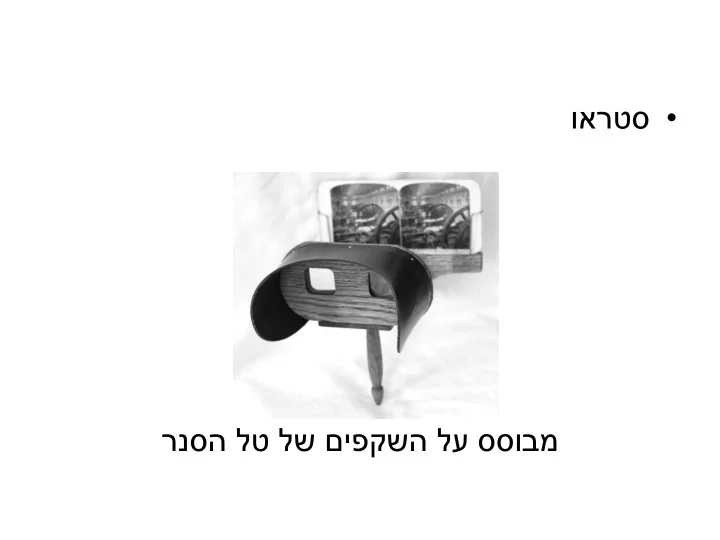
Geometric vision Goal: Recovery - - PowerPoint PPT Presentation

• וארטס

לט לש םיפקשה לע ססובמרנסה

Geometric vision

• Goal: Recovery of 3D structure
• What cues in the image allow us to do this?

Slide credit: Svetlana Lazebnik

Visual Cues

• Shading

3

• B. Leibe

Merle Norman Cosmetics, Los Angeles

Slide credit: Steve Seitz

Visual Cues

• Shading
• Texture

4

• B. Leibe

The Visual Cliff, by William Vandivert, 1960

Slide credit: Steve Seitz

Visual Cues

• Shading
• Texture
• Focus

5

• B. Leibe

From The Art of Photography, Canon

Slide credit: Steve Seitz

Visual Cues

• Shading
• Texture
• Focus
• Perspective

6

• B. Leibe

Slide credit: Steve Seitz

Visual Cues

• Shading
• Texture
• Focus
• Perspective
• Motion

7

Slide credit: Steve Seitz, Kristen Grauman

Figures from L. Zhang http://www.brainconnection.com/teasers/?main=illusion/motion-shape

Our Goal: Recovery of 3D Structure

• We will focus on perspective and motion
• We need multi-view geometry because recovery of

structure from one image is inherently ambiguous

8

• B. Leibe

x X? X? X?

Slide credit: Svetlana Lazebnik

To Illustrate This Point…

• Structure and depth are inherently ambiguous from

single views.

9

• B. Leibe

Slide credit: Svetlana Lazebnik, Kristen Grauman

Perceptual and Sensory Augmented Computing Computer Vision WS 08/09

Stereo Vision

http://www.well.com/~jimg/stereo/stereo_list.html

Slide credit: Kristen Grauman

What Is Stereo Vision?

• Generic problem formulation: given several images of

the same object or scene, compute a representation of its 3D shape

11

• B. Leibe

Slide credit: Svetlana Lazebnik, Steve Seitz

What Is Stereo Vision?

• Generic problem formulation: given several images of

the same object or scene, compute a representation of its 3D shape

12

• B. Leibe

Slide credit: Svetlana Lazebnik, Steve Seitz

What Is Stereo Vision?

• Narrower formulation: given a calibrated binocular

stereo pair, fuse it to produce a depth image

13

• B. Leibe

Image 1 Image 2 Dense depth map

Slide credit: Svetlana Lazebnik, Steve Seitz

Geometry for a Simple Stereo System

• First, assuming parallel optical axes, known camera

parameters (i.e., calibrated cameras):

14

• B. Leibe

Slide credit: Kristen Grauman

15

• B. Leibe

baseline

• ptical center

(left)

• ptical center

(right) Focal length World point Depth of p image point (left) image point (right

Slide credit: Kristen Grauman

Geometry for a Simple Stereo System

• Assume parallel optical axes, known camera parameters

(i.e., calibrated cameras). We can triangulate via:

16

• B. Leibe

Similar triangles (pl, P , pr) an (Ol, P , Or):

Z T f Z x x T

r l

   

l r

x x T f Z  

disparity

Slide credit: Kristen Grauman

Disparity קמועו

תומלצמ

תונומתב הדוקנה ימוקימב לדבה ( disparity ) תומלצמהמ קחרמ( depth )

l r

x x T f Z  

disparity

Depth From Disparity

18

• B. Leibe

Image I(x,y) Image I´(x´,y´) Disparity map D(x,y)

(x´,y´)=(x+D(x,y), y)

General Case With Calibrated Cameras

• The two cameras need not have parallel optical axes.

19

• B. Leibe

vs.

Slide credit: Kristen Grauman, Steve Seitz

Stereo Correspondence Constraints

• Given p in the left image, where can the corresponding

point p’ in the right image be?

20

• B. Leibe

Slide credit: Kristen Grauman

Stereo Correspondence Constraints

• Given p in the left image, where can the corresponding

point p’ in the right image be?

21

• B. Leibe

Slide credit: Kristen Grauman

Stereo Correspondence Constraints

22

• B. Leibe

Slide credit: Kristen Grauman

Stereo Correspondence Constraints

• Geometry of two views allows us to constrain where the

corresponding pixel for some image point in the first view must occur in the second view.

• Epipolar constraint: Why is this useful?
• Reduces correspondence problem to 1D search along conjugate

epipolar lines.

23

• B. Leibe

epipolar plane

epipolar line epipolar line

Slide adapted from Steve Seitz

Epipolar Geometry

24

• Epipolar Plane
• Epipoles
• Epipolar Lines
• Baseline

Slide adapted from Marc Pollefeys

Epipolar Geometry: Terms

• Baseline: line joining the camera centers
• Epipole: point of intersection of baseline with the image

plane

• Epipolar plane: plane containing baseline and world

point

• Epipolar line: intersection of epipolar plane with the

image plane

25

• B. Leibe

Slide credit: Marc Pollefeys

Epipolar Constraint

• Potential matches for p have to lie on the corresponding

epipolar line l’.

• Potential matches for p’ have to lie on the corresponding

epipolar line l.

28

• B. Leibe

http://www.ai.sri.com/~luong/research/Meta3DViewer/EpipolarGeo.html

Slide credit: Marc Pollefeys

Example

29

• B. Leibe

Slide credit: Kristen Grauman

• For a given stereo rig, how do we express the epipolar

constraints algebraically?

33

• B. Leibe

תיחרכהה הצירטמה תיינב

• רידגנ
• בוביס תצירטמ רובע

R , םוקימ ןיב רשקה P אוה תינמיל תילאמשה תוטנידרואוקה תכרעמב:

l

O

r

O P

l



r



l

p

r

p

 

r l

  T O O

 

r l

  P R P T

Rotation Matrix

Express 3d rotation as series of rotations around coordinate axes by angles

   , ,

Overall rotation is product

• f these elementary

rotations:

z y x

R R R R 

Slide credit: Kristen Grauman

תיחרכהה הצירטמה תיינב

• םירוטקוה תשולש ,ו- לע םיאצמנ

רושימה ותוא :רושימה ירלופיפאה

l

O

r

O P

l



r



l

p

r

p

l

P T

( )

l 

P T

Cross Product

• Vector cross product takes two vectors and returns a

third vector that’s perpendicular to both inputs.

• So here, c is perpendicular to both a and b, which

means the dot product = 0.

Slide credit: Kristen Grauman

תיחרכהה הצירטמה תיינב

• םירוטקוה תשולש ,ו- לע םיאצמנ

רושימה ותוא :רושימה ירלופיפאה

• רושימל בצינה רוטקו אוה
• ןאכמ:
• ו תויה-
• יזא:
• לבקנו האושמב ביצנ:

l

O

r

O P

l



r



l

p

r

p

l

P T

( )

l 

P T

 

l

 T P    

T l l

   P T T P

 

r l

  P R P T

T r l

  R P P T

 

T T T r l r l

    R P T P P RT P

Matrix Form of Cross Product

39

Slide credit: Kristen Grauman

תיחרכהה הצירטמה תיינב

• תוצירטמ לפכ תועצמאב בתכשנ

– – רידגנ –לבקנו :

• הצירטמה

E תארקנ תיחרכהה הצירטמה ( Essential Matrix )

 

T T T r l r l

    R P T P P RT P

 

 

T T T r l r x l

   R P T P P R T P

 

x

 E R T

T r l 

P EP

l

O

r

O P

l



r



l

p

r

p

תיחרכהה הצירטמה

• תונותנ תונומתה ירושימב תודוקנו תויה

תוטנידרואוקבמוה,' ףילחנ P ב- p ( דע תוהז ןכש עובקב לפכ ידכל)

• רשיה אוה תינמיה הנומתה רושימב רשי

הדוקנה תא ליכמ יכ חטבומ רשא

• E

תודוקנ תוטנידרואוק ונל תונותנ רשאכ תישומיש רושימב הנומתה.

• הנומתב םילסקיפ תוטנידרואוק שי ונל...

T r l 

p Ep

r l

 u Ep

r

p

Essential Matrix Example: Parallel Cameras

    



]R [T E T I R

x

] , , [ d

0 0 0 0 0 d 0 –d 0

 Ep p

For the parallel cameras, image

• f any point must lie on same

horizontal line in each image plane.

Slide credit: Kristen Grauman

Essential Matrix Example: Parallel Cameras

    



]R [T E T I R

x

] , , [ d

0 0 0 0 0 d 0 –d 0

 Ep p

For the parallel cameras, image

• f any point must lie on same

horizontal line in each image plane.

Slide credit: Kristen Grauman

More General Case

Image I(x,y) Image I´(x´,y´) Disparity map D(x,y)

(x´,y´)=(x+D(x,y), y)

What about when cameras’ optical axes are not parallel?

Slide credit: Kristen Grauman

וארטס תכרעמ לויכ– התידוסיה הצירטמ

תידוסיה הצירטמה

• תידוסיה הצירטמ

Fundamental Matrix F

• ו םעפה ךא תידוסיה הצירטמל הייפואב המוד-

תוטנידרואוקבםילסקיפ

• ו רובע- יתש לש תוימינפ תוצירטמ

תומלצמה

• תועצמאב תידוסיה הצירטמה בושיח"גלא ' הנומש

תודוקנה"

T r l 

p Fp

l

p

r

p

1 T r l  

 F M EM

l

M

l

M

Fundamental matrix

• Relates pixel coordinates in the two views
• More general form than essential matrix: we remove need to

know intrinsic parameters

• If we estimate fundamental matrix from correspondences in

pixel coordinates, can reconstruct epipolar geometry without intrinsic or extrinsic parameters

Grauman

Computing F from correspondences

• Cameras are uncalibrated: we don’t know E or left or right

Mint matrices

• Estimate F from 8+ point correspondences.



 left right p

F p

 

1 int . int ,   



left right EM

M F

Grauman

Computing F from correspondences



 left right p

F p

Each point correspondence generates one constraint on F Collect n of these constraints Solve for f , vector of parameters.

Grauman

Stereo pipeline with weak calibration

So, where to start with uncalibrated cameras?

Need to find fundamental matrix F and the correspondences (pairs of points (u’,v’) ↔ (u,v)).

1) Find interest points in image 2) Compute correspondences 3) Compute epipolar geometry 4) Refine

Example from Andrew Zisserman

1) Find interest points

Stereo pipeline with weak calibration

Grauman

2) Match points only using proximity

Stereo pipeline with weak calibration

Grauman

Putative matches based on correlation search

Grauman

RANSAC for robust estimation of the fundamental matrix

• Select random sample of correspondences
• Compute F using them

– This determines epipolar constraint

• Evaluate amount of support – inliers within threshold distance
• f epipolar line
• Choose F with most support (inliers)

Grauman

Putative matches based on correlation search

Grauman

Pruned matches

• Correspondences consistent with epipolar geometry

Grauman

• Resulting epipolar geometry

Grauman

בושיח רחאל תומאתה תאיצמ F

Stereo image rectification

reproject image planes onto a common plane parallel to the line between optical centers pixel motion is horizontal after this transformation two homographies (3x3 transforms), one for each input image reprojection

Adapted from Li Zhang

In practice, it is convenient if image scanlines are the epipolar lines.

• C. Loop and Z. Zhang. Computing Rectifying Homographies for Stereo Vision. CVPR 1999.

Stereo image rectification: example

Source: Alyosha Efros

Stereo reconstruction: main steps

– Calibrate cameras – Rectify images – Compute disparity – Estimate depth

Grauman

Correspondence problem

Multiple match hypotheses satisfy epipolar constraint, but which is correct?

Figure from Gee & Cipolla 1999

Grauman

Correspondence problem

• Beyond the hard constraint of epipolar geometry, there are

“soft” constraints to help identify corresponding points

– Similarity – Uniqueness – Ordering – Disparity gradient

• To find matches in the image pair, we will assume

– Most scene points visible from both views – Image regions for the matches are similar in appearance

Grauman

Correspondence problem

Source: Andrew Zisserman

Intensity profiles

Source: Andrew Zisserman

Correspondence problem

Source: Andrew Zisserman

Neighborhood of corresponding points are similar in intensity patterns.

Normalized cross correlation

Source: Andrew Zisserman

Correlation-based window matching

Source: Andrew Zisserman

Dense correspondence search

For each epipolar line For each pixel / window in the left image

• compare with every pixel / window on same epipolar line in right image
• pick position with minimum match cost (e.g., SSD, correlation)

Adapted from Li Zhang

Grauman

Textureless regions

Source: Andrew Zisserman

Textureless regions are non-distinct; high ambiguity for matches.

Grauman

Effect of window size

Source: Andrew Zisserman Grauman

Effect of window size

W = 3 W = 20

Figures from Li Zhang

Want window large enough to have sufficient intensity variation, yet small enough to contain only pixels with about the same disparity.

Grauman

Sparse correspondence search

• Restrict search to sparse set of detected features
• Rather than pixel values (or lists of pixel values) use feature descriptor and

an associated feature distance

• Still narrow search further by epipolar geometry

Grauman

םוכיסל :תידוסי הצירטמה ריש!

The Fundamental Matrix Song(360p_H.264-AAC).mp4

םיפקש תורוקמ

• ןיוצש לכ דבלמ , ולא לע םיססובמ םיבר םיפקש

לש:

–

• B. Leibe

–

• K. Grauman

–

• D. Low

–

• S. Lazebnik

–

• A. Torralba

–

• T. Darrell