
SLIDE 1
Generation of Non-Uniform Random Numbers
Refs: Chapter 8 in Law and book by Devroye (watch for typos) Peter J. Haas CS 590M: Simulation Spring Semester 2020
1 / 21
Generation of Non-Uniform Random Numbers Acceptance-Rejection Convolution Method Composition Method Alias Method Random Permutations and Samples Non-Homogeneous Poisson Processes
2 / 21
Acceptance-Rejection
Goal: Generate a random variate X having pdf fX
◮ Avoids computation of F −1(u) as in inversion method ◮ Assumes fX is easy to calculate
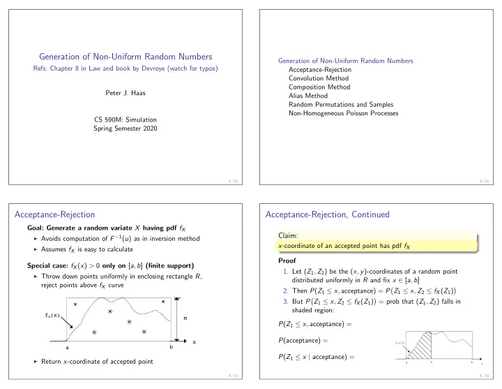
Special case: fX(x) > 0 only on [a, b] (finite support)
◮ Throw down points uniformly in enclosing rectangle R,
reject points above fX curve
fX(x) a b x m
◮ Return x-coordinate of accepted point
3 / 21
Acceptance-Rejection, Continued
Claim:
x-coordinate of an accepted point has pdf fX Proof
- 1. Let (Z1, Z2) be the (x, y)-coordinates of a random point
distributed uniformly in R and fix x ∈ [a, b]
- 2. Then P(Z1 ≤ x, acceptance) = P
- Z1 ≤ x, Z2 ≤ fX(Z1)
- 3. But P
- Z1 ≤ x, Z2 ≤ fX(Z1)
- = prob that (Z1, Z2) falls in
shaded region: P(Z1 ≤ x, acceptance) = P(acceptance) = P(Z1 ≤ x | acceptance) =
4 / 21
x a fX(t) t b