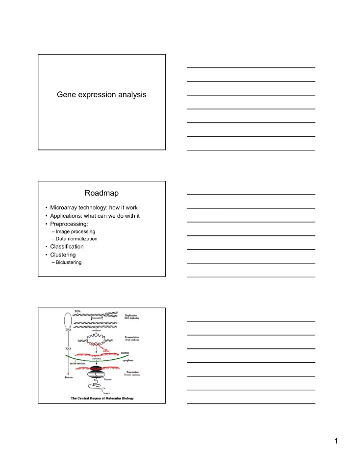
Gene expression analysis Roadmap Microarray technology: how it - PDF document

Gene expression analysis Roadmap • Microarray technology: how it work • Applications: what can we do with it • Preprocessing: – Image processing – Data normalization • Classification • Clustering – Biclustering 1

Gene expression • Gene expression does depend on “space location” and “time location” – Cells from different tissues produce different proteins – Certain genes are expressed only during development or in response to changes to environment, while others are always active ( housekeeping genes) – … DNA microarrays • Monitor the activity of several thousand genes simultaneously • By measuring the amount of mRNA in the cell – One cannot measure directly the mRNA because it is quickly degraded by RNAdigesting enzymes – Use reverse transcription to get cDNA out of the mRNA • DNA “chips” with probes in the order of 10,000- 100,000 are common nowadays • DNA to hybridize Types of microarrays • Affymetrix: lithographic method, 11 pairs of 25-mers (PM, MM) • Oligo/Spotted arrays (cDNA array): pools of oligos attached to a glass slide (60- 70mers) 2

Cartoon version: Before labelling Sample 1 Sample 2 Array 2 Array 1 Before Hybridization Sample 1 Sample 2 Array 2 Array 1 3

After Hybridization Array 2 Array 1 Quantification 4 2 0 3 0 4 0 3 Array 2 Array 1 4

Application domains • Similarity in Expression Patterns of Genes and Experiments (Classification) • Co-regulation of Genes: function and pathways (Clustering) • Network Inference (Modeling) • Type of array: – Control vs. Test – Time-wise – Gene-knockout (perturbation experiments) – … Microarray Data Analysis • Data acquisition and visualization – Image quantification (spot reading) – Dynamic range and spatial effects – Scatter plots – Systematic sources of error • Error models and data calibration • Identification of differentially expressed genes – Fold test – T-test – Correction for multiple testing Comet Comet Tails Dust Tails Dust High Background and Weak Signals Spot overlap High Background and Weak Signals Spot overlap 5

Steps in Images Processing 1. Addressing: locate centers 2. Segmentation: classification of pixels either as signal or background. using seeded region growing). 3. Information extraction: for each spot of the array, calculates signal intensity pairs, background and quality measures. Normalization Why? To correct for systematic differences between samples on the same slide, or between slides, which do not represent true biological variation between samples. Why isn’t “Normalization” Easy? • No ability to read mRNA level directly • Various noise factors → hard to model exactly. • Variable biological settings, experiment dependent. • Need to differentiate between changes caused by biological signal from noise artifacts. 6

Normalization Tools – Current State • Commonly Used: – RMA by Speed Lab – dChip by Li & Wong – GeneChip = MAS5 (Affy. built in tool) • “The Future”: – New Chip design (both Affy. And cDNA) with better probes, better built in controls etc. – New algorithms – facilitating probes GC content (gcRMA), location etc. – New MAS tool is also supposed to incorporate RMA,dChip etc. Microarray Data • Each entry is the 1 2 3 4 5 6 relative expression of G1 0.12 0.43 a gene in test vs. G2 control G3 • Ratio of the color … intensities green/red … (Cy3/Cy5) (spotted) … G 5000 Molecular Classification of Cancer (Golub et al, Science 1999) • Overview: General approach for cancer classification based on gene expression monitoring • The authors address both – Class Prediction (Assignment of tumors to known classes) – Class Discovery (New cancer classes) 7

Cancer Classification • Helps in prescribing necessary treatment • Has been based primarily on morphological appearance • Such approaches have limitations: similar tumors in appearance can be significantly different otherwise • Needed: better classification scheme Cancer Data • Human Patients; Two Types of Leukemia – Acute Myeloid Leukemia – Acute Lymphoblastic Leukemia • Oligo arrays data sets (6817 genes) – Learning Set: 38 bone marrow samples, • 27 ALL, 11 AML • – Test Set: 34 bone marrow samples, • 20 ALL, 14 AML Classification Based on Expression Data • Selecting the most informative genes – Class Distinctors: e.g. express high in AML, but low in ALL – Most informative genes: the neighbors of the distinctor – Used to predict the class of unclassified genes: according to the correlation with the distinctor • Class Prediction (Classification) – Given a new gene, classify it based on the most informative genes – Given a new sample, classify it based on the expression levels of those informative genes • Class Discovery (Clustering) 8

Selecting “Class Distinctor” Genes • The class distincter c is an indicator of the two classes, and is uniformly high in the first (AML), and uniformly low for the second (ALL) • Given another gene g, the correlation is calculated as: µ − µ ( g ) ( g ) = AML ALL P ( g , c ) σ + σ ( ) ( ) g g AML ALL • Where are the µ and σ means and standard deviations of the log of expression levels of gene g for the samples in class AML and ALL. Selecting Informative Genes • Large values of |P(g,c)| indicate strong correlated • Select 50 significantly correlated, 25 most positive and 25 most negative ones • Selecting the top 50 could be possibly bad – If AML gene are more highly expressed than ALL – Unequal number of informative genes for each class Class Prediction • Given a sample, classify it in AML or ALL • Method: – Each of the fixed set of informative genes makes a prediction – The vote is based on the expression level of these genes in the new sample, and the degree of correlation with c – Votes are summed up to determine • The winning class and • The prediction strength (ps) 9

Validity of Class Predictions • Leave-one-out Cross Validation with the initial data (leave one sample out, build the predictor, test the sample) • Validation on an independent data set (strong prediction on 29/34 samples, 100% accuracy) Conclusions • Linear nearest-neighbor discriminators are quick, and identify strong informative signals well • Easy and good biological validation But • Only gross differences in expression are found • Subtler differences cannot be detected • The most informative genes may not be also biologically most informative. It is almost always possible to find genes that split samples into two classes Better classifier? • Support Vector Machines – Inventor: V. N. Vapnik, late seventies – Origin: Theory of Statistical Learning • Have shown promising results in many areas – OCR – Object recognition – Voice recognition – Biological sequence data analysis • What to know more? Ask Chris! 10

Clustering • Given n objects, assign them to groups (clusters) based on their similarity • Unsupervised Machine Learning • Class Discovery • Difficult, and maybe ill-posed problem! Clustering Approaches • Non-Parametric – Agglomerative • Single linkage, average linkage, complete linkage, ward method, … – Divisive • Parametric – K-means, k-medoids, SOM, … • Biclustering • Clustering reveals similar expression patterns, in particular in time-series expression data • This does not mean that a gene of unknown function has the same function as a similarly expressed gene of known function • Genes of similar expression might be similarly regulated 11

How To Choose the Right Clustering? • Data Type: – Single array measurement? – Series of experiments • Quality of Clustering • Code Availability • Features of the Methods – Computing averages (sometimes impossible or too slow) – Sensitivity to Perturbation and other indices – Properties of the clusters – Speed – Memory Hierarchical Clustering • Input: Data Points, x 1 ,x 2 ,…,x n • Output:Tree – the data points are leaves – Branching points indicate similarity between sub- trees – Horizontal cut in the tree produces data clusters 1 2 4 5 3 4 5 1 2 3 General Algorithm 1. Place each element in its own cluster, Ci={xi} 2. Compute (update) the merging cost between every pair of elements in the set of clusters to find the two cheapest to merge clusters Ci, Cj, 3. Merge Ci and Cj in a new cluster Cij which will be the parent of Ci and Cj in the result tree. 4. Go to (2) until there is only one set remaining 12