Gaussian Quiz H 1 y 2 y 1 y 3 1 . Assuming that the variables y 1 , y - - PDF document

SLIDE 1

Preamble to ‘The Humble Gaussian Distribution’. David MacKay 1

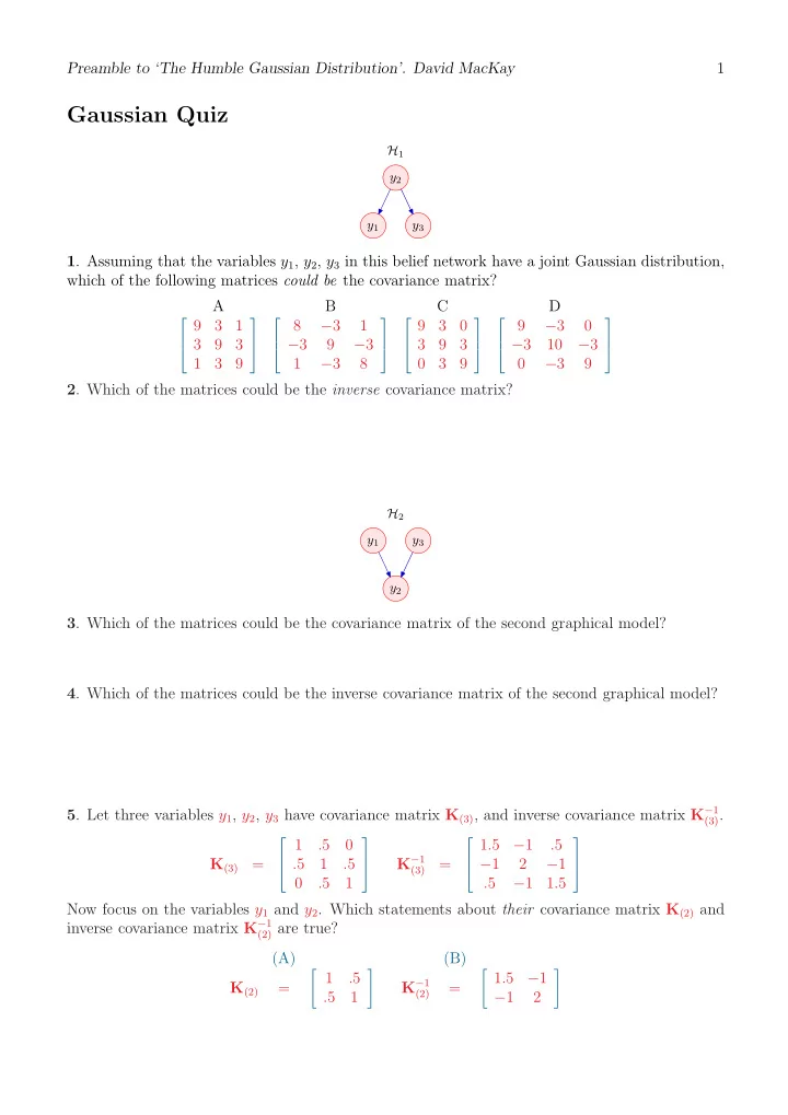
Gaussian Quiz

y1 y3 y2 H1

• 1. Assuming that the variables y1, y2, y3 in this belief network have a joint Gaussian distribution,

which of the following matrices could be the covariance matrix? A B C D

  

9 3 1 3 9 3 1 3 9

     

8 −3 1 −3 9 −3 1 −3 8

     

9 3 3 9 3 3 9

     

9 −3 −3 10 −3 −3 9

  

• 2. Which of the matrices could be the inverse covariance matrix?

y1 y3 y2 H2

• 3. Which of the matrices could be the covariance matrix of the second graphical model?
• 4. Which of the matrices could be the inverse covariance matrix of the second graphical model?
• 5. Let three variables y1, y2, y3 have covariance matrix K(3), and inverse covariance matrix K−1

(3).

K(3) =

  

1 .5 .5 1 .5 .5 1

  

K−1

(3)

=

  

1.5 −1 .5 −1 2 −1 .5 −1 1.5

  

Now focus on the variables y1 and y2. Which statements about their covariance matrix K(2) and inverse covariance matrix K−1

(2) are true?

(A) (B) K(2) =

• 1

.5 .5 1

• K−1

(2)

=

• 1.5

−1 −1 2

SLIDE 2

The Humble Gaussian Distribution

David J.C. MacKay Cavendish Laboratory Cambridge CB3 0HE United Kingdom June 11, 2006 – Draft 1.0

Abstract These are elementary notes on Gaussian distributions, aimed at people who are about to learn about Gaussian processes. I emphasize the following points. What happens to a covariance matrix and inverse covariance matrix when we omit a variable. What it means to have zeros in a covariance matrix. What it means to have zeros in an inverse covariance matrix. How probabilistic models expressed in terms of ‘energies’ relate to Gaussians. Why eigenvectors and eigenvalues don’t have any fundamental status.

1 Introduction

Let’s chat about a Gaussian distribution with zero mean, such as P(y) = 1 Z e

−1

2y

TAy,

(1) where A = K−1 is the inverse of the covariance matrix, K, and Z = [det 2πK]1/2. I’m going to emphasize dimensions throughout this note, because I think dimension-consciousness enhances understanding.1 I’ll write K =

  

K11 K12 K13 K12 K22 K23 K13 K23 K33

  

(4)

1It’s conventional to write the diagonal elements in K as σ2 i and the offdiagonal elements as σij. For example

K =   σ2

1

σ12 σ13 σ12 σ2

2

σ23 σ13 σ23 σ2

3

  (2) A confusing convention, since it implies that σij has different dimensions from σi, even if all axes i, j have the same dimensions! Another way of writing an off-diagonal coefficient is Kij = ρijσiσj, (3) where ρ is the correlation coefficient between i and j. This is a better notation since it’s dimensionally consistent in the way it uses the letter σ. But I will stick with the notation Kij.

2

SLIDE 3

The definition of the covariance matrix is Kij = yiyj (5) so the dimensions of the element Kij are (dimensions of yi) times (dimensions of yj).

1.1 Examples

Let’s work through a few graphical models.

y1 y3 y2 H1 y1 y3 y2 H2

Example 1 Example 2 1.1.1 Example 1 Maybe y2 is the temperature outside some buildings (or rather, the deviation of the outside temperature from its mean), and y1 is the temperature deviation inside building 1, and y3 is the temperature inside building 3. This graphical model says that if you know the outside temperature y2 then y1 and y3 are independent. Let’s consider this generative model: y2 = ν2 (6) y1 = w1y2 + ν1 (7) y3 = w3y2 + ν3, (8) where {νi} are independent normal variables with variances {σ2

i }.

Then we can write down the entries in the covariance matrix, starting with the diagonal entries K11 = y1y1 = (w1ν2 + ν1)(w1ν2 + ν1) = w2

1ν2 2 + 2w1ν1ν2 + ν1 2 = w2 1σ2 2 + σ2 1

(9) K22 = σ2

2

(10) K33 = w2

3σ2 2 + σ2 3

(11) So we can fill in this much: K =

  

K11 K12 K13 K12 K22 K23 K13 K23 K33

   =   

w2

1σ2 2 + σ2 1

σ2

2

w2

3σ2 2 + σ2 3

  

(12) The off diagonal terms are K12 = y1y2 = (w1ν2 + ν1)(ν2) = w1σ2

2

(13) (and similarly for K23) and K13 = y1y3 = (w1ν2 + ν1)(w3ν2 + ν3) = w1w3σ2

2

(14) 3

SLIDE 4

So the covariance matrix is: K =

  

K11 K12 K13 K12 K22 K23 K13 K23 K33

   =   

w2

1σ2 2 + σ2 1

w1σ2

2

w1w3σ2

2

σ2

2

w3σ2

2

w2

3σ2 2 + σ2 3

  

(15) (where the remaining blank elements can be filled in by symmetry). Now let’s think about the inverse covariance matrix. One way to get to it is to write down the joint distribution. P(y1, y2, y3 | H1) = P(y2)P(y1 | y2)P(y3 | y2) (16) = 1 Z2 exp

• − y2

2

2σ2

2

1

Z1 exp

• −(y1 − w1y2)2

2σ2

1

1

Z3 exp

• −(y3 − w3y2)2

2σ2

3

• (17)

We can now collect all the terms in yiyj. P(y1, y2, y3) = 1 Z′ exp

• − y2

2

2σ2

2

− (y1 − w1y2)2 2σ2

1

− (y3 − w3y2)2 2σ2

3

• =

1 Z′ exp

• −y2

2

1

2σ2

2

+ w2

1

2σ2

1

+ w2

3

2σ2

3

• − y2

1

1 2σ2

1

+ 2y1y2 w1 2σ2

1

− y2

3

1 2σ2

3

+ 2y3y2 w3 2σ2

3

• =

1 Z′ exp

         

−1 2

• y1

y2 y3

• 

        

1 σ2

1

−w1 σ2

1

−w1 σ2

1

1

σ2

2

+ w2

1

σ2

1

+ w2

3

σ2

3

• −w3

σ2

3

−w3 σ2

3

1 σ2

3

                 

y1 y2 y3

                 

So the inverse covariance matrix is K−1 =

         

1 σ2

1

−w1 σ2

1

−w1 σ2

1

1

σ2

2

+ w2

1

σ2

1

+ w2

3

σ2

3

• −w3

σ2

3

−w3 σ2

3

1 σ2

3

         

The first thing I’d like you to notice here is the zeroes. [K−1]13 = 0. The meaning of a zero in an inverse covariance matrix (at location i, j) is conditional on all the other variables, these two variables i and j are independent. Next, notice that whereas y1 and y2 were positively correlated (assuming w1 > 0), the coefficient [K−1]12 is negative. It’s common that a covariance matrix K in which all the elements are non- negative has an inverse that includes some negative elements. So positive off-diagonal terms in the covariance matrix always describe positive correlation; but the off-diagonal terms in the inverse covariance matrix can’t be interpreted that way. The sign of an element (i, j) in the inverse covariance matrix does not tell you about the correlation between those two variables. For example, remember: there is a zero at [K−1]13. But that doesn’t mean that variables y1 and y3 are uncorrelated. Thanks to their parent y2, they are correlated, with covariance w1w3σ2

2.

The off-diagonal entry [K−1]ij in an inverse covariance matrix indicates how yi and yj are correlated if we condition on all the other variables apart from those two: if [K−1]ij < 0, they are positively correlated, conditioned on the others; if [K−1]ij > 0, they are negatively correlated. 4

SLIDE 5

The inverse covariance matrix is great for reading out properties of conditional distributions in which we condition on all the variables except one. For example, look at

• K−1

11 = 1

σ2

1

; if we know y2 and y3, then the probability distribution of y1 is Gaussian with variance 1/ [K−1] 11. That one was easy. Look at

• K−1

22 =

1

σ2

2

+ w2

1

σ2

1

+ w2

3

σ2

3

• . if we know y1 and y3, then the probability distribution
• f y2 is Gaussian with variance

1 [K−1] 22 = 1 1 σ2

2

+ w2

1

σ2

1

+ w2

3

σ2

3

. (18) That’s not so obvious, but it’s familiar if you’ve applied Bayes theorem to Gaussians – when we do inference of a parent like y2 given its children, the inverse-variances of the prior and the likelihoods

• add. Here, the parent variable’s inverse variance (also known as its precision) is the sum of the

precision contributed by the prior

1 σ2

2 , the precision contributed by the measurement of y1, w2 1

σ2

1 , and

the precision contributed by the measurement of y3, w2

3

σ2

3 .

The off-diagonal entries in K tell us how the mean of [the conditional distribution of one variable given the others] depends on [the others]. Let’s take variable y3 conditioned on the other two, for example. P(y3 | y1, y2, H1) ∝ P(y1, y2, y3 | H1) ∝ 1 Z′ exp

        

−1 2

• y1

y2 y3

• 

       

1 σ2

1

−w1 σ2

1

−w1 σ2

1

1

σ2

2

+ w2

1

σ2

1

+ w2

3

σ2

3

• −w3

σ2

3

−w3 σ2

3

1 σ2

3

                

y1 y2 y3

                

Let’s highlight in Blue the terms y1, y2 that are fixed and known and uninteresting, and highlight in Green everything that is multiplying the interesting term y3. P(y3 | y1, y2, H1) ∝ P(y1, y2, y3 | H1) ∝ 1 Z′ exp

        

−1 2

• y1

y2 y3

• 

       

1 σ2

1

−w1 σ2

1

−w1 σ2

1

1

σ2

2

+ w2

1

σ2

1

+ w2

3

σ2

3

• −w3

σ2

3

−w3 σ2

3

1 σ2

3

                

y1 y2 y3

                

All those blue multipliers in the central matrix aren’t achieving anything. We can just ignore them (and redefine the constant of proportionality). For the benefit of anyone with a colour-blind printer, here it is again: P(y3 | y1, y2, H1) ∝ exp

      

−1 2

• y1

y2 y3

• 

     

−w3 σ2

3

−w3 σ2

3

1 σ2

3

            

y1 y2 y3

            

5

SLIDE 6

P(y3 | y1, y2, H1) ∝ exp

• −1

2 1 σ2

3

[y3]2 − [y3]

• 0 × y1 − w3

σ2

3

× y2

• We obtain the mean by completing the square. 2

P(y3 | y1, y2, H1) ∝ exp

      

−1 2 1 σ2

3

     y3 −

• 0 × y1 + w3

σ2

3

× y2

• 1

σ2

3

     

2

     

In this case, this all collapses down, of course, to P(y3 | y1, y2, H1) ∝ exp

• −1

2 1 σ2

3

[y3 − w3y2]2

• ,

(19) as defined in the original generative model (8). In general, the offdiagonal coefficients K−1 tell us the sensitivity of [the mean of the conditional distribution] to the other variables. µy3 | y1,y2 = −K−1

13 y1 − K−1 23 y2

K−1

33

(20) So the conditional mean of y3 is a linear function of the known variables, and the offdiagonal entries in K−1 tell us the coefficients in that linear function.

y1 y3 y2 H1 y1 y3 y2 H2

Example 1 Example 2

1.2 Example 2

Here’s another example, where two parents have one child. For example, the price of electricity y2 from a power station might depend on the price of gas, y1, and the price of carbon emission rights, y3.

y1 y3 y2 H2

Example 2

2‘Completing the square’ is 1 2ay2 − by = 1 2a(y − b/a)2 + constant.

6

SLIDE 7

y2 = w1y1 + w3y3 + ν2 (21) Note that the units in which gas price, electricity price, and carbon price are measured are all different (pounds per cubic metre, pennies per kWh, and euros per tonne, for example). So y1, y3, and y3 have different dimensions from each other. Most people who do data modelling treat their data as ‘just numbers’, but I think it is a useful discipline to keep track of dimensions and to carry out only dimensionally valid operations. [Dimensionally valid operations satisfy the two rules of dimensions: (1) only add, subtract and compare quantities that have like dimensions; (2) arguments of all functions like exp, log, sin must be dimensionless. Rule 2 is really just a special case of rule 1, since exp(x) = 1 + x + x2 + . . ., so to satisfy rule 1, the dimensions of x must be the same as the dimensions of 1.] What is the covariance matrix? Here we assume that the parent variables y1 and y3 are uncorrelated. The covariance matrix is K =

  

K11 K12 K13 K12 K22 K23 K13 K23 K33

   =   

σ2

1

w1σ2

1

σ2

2 + w2 1σ2 1 + w2 3σ2 3

w3σ2

3

σ2

3

  

(22) Notice the zero correlation between the uncorrelated variables (1, 3). What do you think the (1, 3) entry in the inverse covariance matrix will be? Let’s work it out in the same way as before. The joint distribution is P(y1, y2, y3 | H2) = P(y1)P(y3)P(y2 | y1, y3) (23) = 1 Z1 exp

• − y2

1

2σ2

1

1

Z3 exp

• − y2

3

2σ2

3

1

Z2 exp

• −(y2 − w1y1 − w3y3)2

2σ2

2

• (24)

We collect all the terms in yiyj. P(y1, y2, y3) = 1 Z′ exp

• − y2

1

2σ2

1

− y2

3

2σ2

3

− (y2 − w1y1 − w3y3)2 2σ2

2

• =

1 Z′ exp

• −y2

1

1

2σ2

1

+ w2

1

2σ2

2

• − y2

2

1 2σ2

2

+ 2y1y2 w1 2σ2

1

−y2

3

1

2σ2

3

+ w2

3

2σ2

2

• + 2y3y2

w3 2σ2

2

− 2y3y1 w1w3 2σ2

2

• =

1 Z′ exp

         

−1 2

• y1

y2 y3

• 

         1

2σ2

1

+ w2

1

σ2

2

• −w1

σ2

2

+w1w3 σ2

2

−w1 σ2

2

1 σ2

2

−w3 σ2

2

+w1w3 σ2

2

−w3 σ2

2

1

2σ2

3

+ w2

3

σ2

2

• 

                

y1 y2 y3

                 

So the inverse covariance matrix is K−1 =

          1

2σ2

1

+ w2

1

σ2

2

• −w1

σ2

2

+w1w3 σ2

2

−w1 σ2

2

1 σ2

2

−w3 σ2

2

+w1w3 σ2

2

−w3 σ2

2

1

2σ2

3

+ w2

3

σ2

2

• 

        

(25) 7

SLIDE 8

Notice (assuming w1 > 0 and w3 > 0) that the offdiagonal term connecting a parent and a child [K−1]12 is negative and the offdiagonal term connecting the two parents [K−1]13 is positive. This positive term indicates that, conditional on all the other variables (i.e., y2), the two parents y1 and y3 are anticorrelated. That’s ‘explaining away’. Once you know the price of electricity was average, for example, you can deduce that if gas was more expensive than normal, carbon probably was less expensive than normal.

2 Omission of one variable

Consider example 1.

y1 y3 y2 H1

Example 1 The covariance matrix of all three variables is: K =

  

K11 K12 K13 K12 K22 K23 K13 K23 K33

   =   

w2

1σ2 2 + σ2 1

w1σ2

2

w1w3σ2

2

σ2

2

w3σ2

2

w2

3σ2 2 + σ2 3

  

(26) If we decide we want to talk about the joint distribution of just y1 and y2, the covariance matrix is simply the sub-matrix: K2 =

• K11

K12 K12 K22

• =
• w2

1σ2 2 + σ2 1

w1σ2

2

σ2

2

• (27)

This follows from the definition of the covariance, Kij = yiyj. (28) The inverse covariance matrix, on the other hand, does not change in such a simple way. The 3 × 3 inverse covariance matrix was: K−1 =

         

1 σ2

1

−w1 σ2

1

−w1 σ2

1

1

σ2

2

+ w2

1

σ2

1

+ w2

3

σ2

3

• −w3

σ2

3

−w3 σ2

3

1 σ2

3

         

When we work out the 2 × 2 inverse covariance matrix, all the Blue terms that originated from the child y3 are lost. So we have K−1

2

=

    

1 σ2

1

−w1 σ2

1

−w1 σ2

1

1

σ2

2

+ w2

1

σ2

1

• 

   

8

SLIDE 9

Specifically, notice that

• K−1

2

• 22 is different from the (2, 2) entry in the three by three K−1.

We conclude: Leaving out a variable leaves K unchanged but changes K−1. This conclusion is important for understanding the answer to the question, ‘When working with Gaussian processes, why not parameterize the inverse covariance instead of the covariance function?’ The answer is: you can’t write down the inverse covariance associated with two points! The inverse covariance depends capriciously on what the other variables are.

3 Energy models

Sometimes people express probabilistic models in terms of energy functions that are minimized in the most probable configuration. For example, in regression with cubic splines, a regularizer is defined which describes the energy that a steel ruler would have if bent into the shape of the curve. Such models usually have the form: P(y) = 1 Z e−E(y) T , (29) and in simple cases, the energy E(y) may be a quadratic function of y, such as E(y) = −

• i<j

Jijyiyj +

• i

aiy2

i

(30) If so, then the distribution is a Gaussian (just like (1)), and the ‘couplings’ Jij are minus the coefficients in the inverse covariance matrix. As a simple example, consider a set of three masses coupled by springs, and subjected to thermal perturbations.

y1 y2 y3 k01 k12 k23 k34

Three masses, four springs The equilbrium positions are (y1, y2, y3, y4) = (0, 0, 0, 0), and the spring constants are kij. The extension of the second spring is y2 − y1. The energy of this system is E(y) = 1 2k01y2

1 + 1

2k12(y2 − y1)2 + 1 2k23(y3 − y2)2 + 1 2k34y2

3

= 1 2

• y1

y2 y3

• 

 

k01 + k12 −k12 −k12 k12 + k23 −k23 −k23 k23 + k34

     

y1 y2 y3

  

So at temperature T, the probability distribution of the displacements is Gaussian with inverse covariance matrix 1 T

  

k01 + k12 −k12 −k12 k12 + k23 −k23 −k23 k23 + k34

  

(31) Notice that there are 0 entries between displacements y1 and y3, the two masses that are not directly coupled by a spring. 9

SLIDE 10

y1 y2 y3 y4 y5 k k k k k k

Figure 1. Five masses, six springs

So inverse covariance matrices are sometimes very sparse. If we have five masses in a row connected by identical springs k for example, then K−1 = k T

       

2 −1 −1 2 −1 −1 2 −1 −1 2 −1 −1 2

       

. (32) But this sparsity doesn’t carry over to the covariance matrix, which is K = T k

       

0.83 0.67 0.50 0.33 0.17 0.67 1.33 1.00 0.67 0.33 0.50 1.00 1.50 1.00 0.50 0.33 0.67 1.00 1.33 0.67 0.17 0.33 0.50 0.67 0.83

       

. (33)

4 Eigenvectors and eigenvalues are meaningless

There seems to be a knee-jerk reaction when people see a square matrix: ‘what are its eigenvec- tors?’ But here, where we are discussing quadratic forms, eigenvectors and eigenvalues have no fundamental status. They are dimensionally invalid objects. Any algorithm that features eigen- vectors either didn’t need to do so, or shouldn’t have done so. (I think the whole idea of principal component analysis is misguided, for example.) Hang on, you say, what about the three masses example? Don’t those three masses have meaningful normal modes? Yes, they do, but those modes are not the eigenvectors of the spring matrix (31). Remember, I didn’t tell you what the masses of the masses were! I’m not saying that eigenvectors are never meaningful. What I’m saying is, in the context of quadratic forms 1 2y

TAy,

(34) eigenvectors are meaningless and arbitrary. Consider a covariance matrix describing the correlation between something’s mass y1 and its length y2. K =

• K11

K12 K12 K22

• (35)

The dimensions of K11 are mass-squared. K11 might be measured in kg2, for example. The dimensions of K12 ≡ y1y2 are mass times length. K12 might be measured in kg m, for example. Here’s an example, which might describe the correlation between weight and height of some animals in a survey. K =

• K11

K12 K12 K22

• =
• 10000 kg2

70 kg m 70 kg m 1 m2

• (36)

10

SLIDE 11

• 100

100 200

• 200
• 100

100 200 length / cm mass / kg

• 1

1 2

• 200
• 100

100 200 length / m mass / kg

Figure 2. Dataset with its ‘eigenvectors’. As the text explains, the eigenvectors of covariance matrices are meaningless and arbitrary.

The knee-jerk reaction is “let’s find the principal components of our data”, which means “ignore those silly dimensional units, and just find the eigenvectors of

• 10000

70 70 1

• . But let’s consider

what this means. An eigenvector is a vector satisfying

• 10000 kg2

70 kg m 70 kg m 1 m2

• e = λe.

(37) By asking for an eigenvector, we are imagining that two equations are true – first, the top row: 10000 kg2 e1 + 70 kg m e2 = λe1, (38) and, second, the bottom row: 70 kg m e1 + 1 m2 e2 = λe2. (39) These expressions violate the rules of dimensions. Try all you like, but you won’t be able to find dimensions for e1, e2, and λ such that rule 1 is satisfied. No, no, the matlab lover says, I leave out the dimensions, and I get: > [e,v] = eig(s) e = 0.0070002

• 0.9999755

v = 5.0998e-01 0.0000e+00

• 0.9999755
• 0.0070002

0.0000e+00 1.0000e+04 I notice that the eigenvectors (0.007, −0.9999), and (0.9999, 0.007), which are almost aligned with the coordinate axes. Very interesting! I also notice that the eigenvalues are 104 and 0.5. What an interestingly large eigenvalue ratio! Wow, that means that there is one very big principal component, and the second one is much smaller. Ooh, how interesting. 11

SLIDE 12

But this is nonsense. If we change the units in which we measure length from m to cm then the covariance matrix can be written: K =

• K11

K12 K12 K22

• =
• 10000 kg2

7000 kg cm 7000 kg cm 10000 cm2

• (40)

This is exactly the same covariance matrix of exactly the same data. But the eigenvectors and eigenvalues are now: e =

• 0.70711

0.70711 v = 3000 0.70711 0.70711 17000 Figure 2 illustrates this situation. On the left, a data set of masses and lengths measured in metres. The arrows show the ‘eigenvectors’. (The arrows don’t look ‘orthogonal’ in this plot because a step of one unit on the x-axis happens to cover less paper than a step of one unit on the y-axis.) On the right, exactly the same data set but with lengths measured in centimetres. The arrows show the ‘eigenvectors’. In conclusion, eigenvectors of the matrix in a quadratic form are not fundamentally meaningful. [Properties of that matrix that are meaningful include its determinant.]

4.1 Aside

This complaint about eigenvectors comes hand in hand with another complaint, about ‘steepest descent’. A steepest descent algorithm is dimensionally invalid. A step in a parameter space does not have the same dimensions as a gradient. To turn a gradient into a sensible step direction, you need a metric. The metric defines how ‘big’ a step is (in rather the same way that when gnuplot plotted the data above, it chose a vertical scale and a horizontal scale). Once you know how big alternative steps are, it becomes meaningful to take the step that is ‘steepest’ (that is, it’s the direction with the biggest change in function value per unit ‘distance’ moved). Without a metric, steepest descents algorithms are not covariant. That is, the algorithm would behave differently if you just changed the units in which one parameter is measured.

Appendix: Answers to quiz

For the first four, you can quickly guess the answers based on whether the (1, 3) entries are zero

• r not. For a careful answer you should also check that the matrices really are positive definite

(they are) and that they are realisable by the respective graphical models (which isn’t guaranteed by the preceding constraints).

• 1. A and B
• 2. C and D
• 3. C and D
• 4. A and B
• 5. A is true, B is false.

12