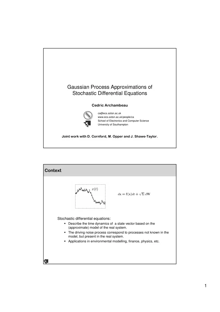
Gaussian Process Approximations of Stochastic Differential Equations - PDF document

Gaussian Process Approximations of Stochastic Differential Equations ����������������� ca@ecs.soton.ac.uk www.ecs.soton.ac.uk/people/ca School of Electronics and Computer Science University of Southampton ������������������������������������� �������������������� ����� � x ( t ) Stochastic differential equations: � Describe the time dynamics of a state vector based on the (approximate) model of the real system. � The driving noise process correspond to processes not known in the model, but present in the real system. � Applications in environmental modelling, finance, physics, etc. 1

���!��������������"����������������������������� � Numerical weather prediction models: � Based on the discretisation of coupled partial differential equations � Dynamical models are imperfect � State vectors have typically dimension O (10 � ) . � Large number of data, but relatively few compared to dimension � Previous approaches consider the models as deterministic or propagate only mean forward in time. � Recent work attempts propagating uncertainty as well (e.g., approximate Monte Carlo methods). � Most approaches do not deal with estimating unknown model parameters. � We focus on a GP and a variational approximation and expect it can be applied to very large models, by exploiting localisation, hierarchical models and sparse representations. �#��#��� � Basic setting � Probability measures and state paths � GP approximation of the posterior measure � Variational approximation of the posterior measure 2

$�%���%�����! � Stochastic differential equation: � Noise model (likelihood): &'��(�%�����%������������������)������ � Discrete time form of Ito’s SDE: with � The Wiener process is a Gaussian stochastic process with independent increments (if not overlapping): 3

*��������������%���%����%���������% � The nonlinear function f induces a prior non-Gaussian probability measure over state paths in time: � Inference problem: +��%%��������� �����������������%����������%��� � Approximate the posterior measure by a Gaussian process: � Replace the non-Gaussian Markov process by a Gaussian one: with � Minimize Kullback-Leibler divergence along the state path: with 4

��������!�����,-���#��!���������!���%��������� � Discretized SDEs: � Probability density of the discrete time path: p ( x �� K ) = � k N ( x k �� | x k + f ( x k )∆ t, Σ ∆ t ) q ( x �� K ) = � k N ( x k �� | x k + f L ( x k , t k )∆ t, Σ ∆ t ) � KL along a discrete path: KL [ q ( x �� K ) � p sde ( x �� K )] � d x k q ( x k ) � d x k �� q ( x k �� | x k ) ln q � � � �� | � � � = � k p � � � �� | � � � � � = � d x k q ( x k ) ( f − f L ) � Σ − � ( f − f L )∆ t k � � Pass to a continuum by taking the limit . ∆ t → 0 +��%%���������%%���%�������������% � GP approximation of the prior process: � Compute induced two-time kernel by solving its ordinary differential equations: � Posterior moments (standard GP regression): 5

. ������/"� ���%�����0�������� �����%% � Prior process: f ( x ) = − γx � Solution to the kernel ODE: K ( t � , t � ) = K ( t � , t � ) exp {− A ( t � − t � ) } � Resulting induced kernel: K ( t � , t � ) = σ � � γ exp {− γ | t � − t � |} Evidence Ornstein-Uhlenbeck kernel x ( t ) γ = 1 ln p ( D ) γ t 6

. ������1" ������������%�%��� � Prior process: U ( x ) x ( t ) � Stationary kernel: with Stationary (OU) kernel Squared exponential kernel x ( t ) x ( t ) t t ln p ( D ) α 7

2���������� ����� �����������������%�������������% � Why? � Constraint on the mean and covariance of the marginals: � Seeking for the stationary points of the Lagrangian leads to: ����%%�����%�������!���!������ Repeat until convergence: Forward propagation of the mean and the covariance. 1. Backward propagation of the Lagrange multipliers: 2. Use jump conditions when there’s an observation: Update the parameters of the approximate SDE: 3. 8

. ������/" ���%�����0�������� �����%% f ( x ) = − γx f L ( x ) = − Ax + b . ������1" ������������%�%��� f ( x ) = 4 x (1 − x � ) 1 FW-BW sweep GP initialization 2 FW-BW sweep Ensemble Kalman smoother − ln Z (Eyinck, et al. , 2002) # sweeps 9

������%��� � Proper modelling requires to take into account that the prior process is a non-Gaussian process. � A key quantity in the energy function is the KL divergence between processes over a time interval (i.e., between probability measures over paths!) � Unlike in standard GP regression, the feature that the process is infinite dimensional plays a role in the inference. � These results were preliminary ones, but the framework is a general one (not limited to smoothing in time). 10