Fundamental Equations Bayes decision rule: = arg max { P ( | O ) } - - PowerPoint PPT Presentation

Fundamental Equations

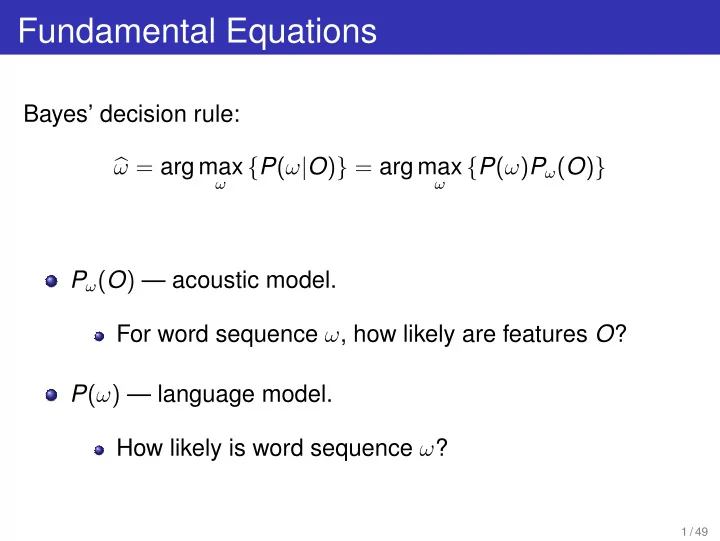
Bayes’ decision rule:

• ω = arg max

ω

{P(ω|O)} = arg max

ω

{P(ω)Pω(O)} Pω(O) — acoustic model. For word sequence ω, how likely are features O? P(ω) — language model. How likely is word sequence ω?

1 / 49

Lecture 9

Speaker Adaptation Michael Picheny, Bhuvana Ramabhadran, Stanley F . Chen, Markus Nussbaum-Thom

Watson Group IBM T.J. Watson Research Center Yorktown Heights, New York, USA {picheny,bhuvana,stanchen,nussbaum}@us.ibm.com

8 April 2016

Where Are We?

[0]

1

Introduction

2

Segmentation and Clustering

3

Maximum Likelihood Linear Regression

4

Feature based Maximum Likelihood Linear Regression

5

Speaker Adaptive Training

3 / 49

Problem: Sources of Variability

gender: male / female age: young / old accents: Texas, South-Carolina environment noise: office, car, shopping mall different types of microphone channel characteristics: high-quality, telephone, mobile phone Question: Are all these effects covered in training ?

4 / 49

Changing Conditions (I)

Training data: Should represent test data adequately. Problem: There will always be new speakers or conditions. Consequence: What will happen ? Recognition performance drops.

5 / 49

Changing Conditions (II)

Why does the performance drop ? The features are different from training. Situation in training: Larger amount data for a specific set of speakers. Situation in recognition: Small amount of data from a target speaker. What can we do ?

6 / 49

Adaptation vs. Normalization

What can we do to overcome the mismatch between training and recognition ? Change features O or the acoustic model P(O|ω, θ). O: feature sequence. ω: word sequence. θ: free model parameters. Model-based – Feature-based: Modify model to better fit the features ⇒ adaptation. Transform features to better fit model ⇒ normalization.

7 / 49

Terminology

Speaker: Rather a concept for different signal conditions. Speaker-independent (SI) system: trained on complete data. Speaker-dependent (SD) system: trained on all the data per speaker. Speaker-adaptive (SA) system: adapted SI system using the speaker dependent data.

8 / 49

Adaptation/Normalization Types

Supervised vs. Unsupervised: Is correct transcription of utterance available at test time ? Batch vs. Incremental adaptation/normalization: Whole vs. small (time critical) portion of the test data is available. Online vs. Offline system: Real-time demand vs. No time restriction.

9 / 49

Question answer (I)

What is the concept of a speaker ? Are all speaker covered in the training data ? What happens ? How do we approach the problem of unseen speaker ? Supervised vs. unsupervised ? Batch vs. Incremental ?

10 / 49

Strategies Summary

Goal: Fit acoustic model/features to speaker. Use new acoustic adaptation data from the current speaker. Model-based – Feature-based: Modify model to better fit the features ⇒ adaptation. Transform features to better fit model ⇒ normalization. Supervised – Unsupervised: Transcription is available for adaptation ⇒ supervised. No transcription is available ⇒ unsupervised. Training: Normalization/Adaptation also in training ⇒ Speaker Adaptive Training (SAT). Incremental – Batch: adaptation only on small parts ⇒ incremental. adaptation on all data ⇒ batch.

11 / 49

Transformation of a Random Variable

Consider a random variable O: with density P(O) and transform O

′ = f(O) (assume f can be inverted)

Then the density P(O

′) is:

P(O

′) =

1

• d f(O)

d O

• P(f −1(O

′)) =

1

• d f(O)

d O

• P(O)

with Jacobian determinant:

• d f(O)

d O

• r equivalent:

P(O) =

• d f(O)

d O

• P(O

′) 12 / 49

Supervised Normalization and Adaptation

Estimation of adaptation parameters Model based: θ′ = f(θ, Φ) ˆ Φ = arg max

Φ

P(O|ω, θ′) Feature based: O′ = f(O, Φ) (| · | is the Jacobi matrix) ˆ Φ = arg max

Φ

• d f(O, Φ)

d O

• P(O′|ω, θ)

Correct transcript ω of adaptation data is given.

13 / 49

Unsupervised Normalization and Adaptation

Estimation of adaptation parameters and generation of adaptation word sequence. Model based: θ′ = f(θ, Φ) (ˆ ω, ˆ Φ) = arg max

ω,Φ P(O|ω, θ′).

Feature based: O′ = f(O, Φ) (ˆ ω, ˆ Φ) = arg max

ω,Φ

• d f(O, Φ)

d O

• P(O′|ω, θ).

In practice infeasable. In practice transcript ω of adaptation data is approximated.

14 / 49

Unsupervised Normalization and Adaptation: First Best Approximation

First-best approximation A speaker independent system generates the first best

• utput.

Estimation is performed exactly as in the supervised case, but use first pass output as transcription. Most popular method.

15 / 49

Unsupervised Normalization and Adaptation: Word Graph Approximation

Word graph based approximation A first pass recognition generates a word graph. Use the forward-backward algorithm as in the supervised case based on the word graph. Weighted accumulation.

THE THIS THUD DIG DOG DOG DOGGY ATE EIGHT MAY MY MAY

16 / 49

Question answer (II)

Superprvised vs. Unsupervised adaptation ? Approximations ?

17 / 49

Where Are We?

[0]

1

Introduction

2

Segmentation and Clustering

3

Maximum Likelihood Linear Regression

4

Feature based Maximum Likelihood Linear Regression

5

Speaker Adaptive Training

18 / 49

Online System

Objective: generate transcription from audio in real time. The audio has multiple unknown speakers and conditions. Requires fast adaptation with very little data (a couple of seconds). Can benefit from incremental adaptation which continuously updates the adaptation for new data.

19 / 49

Offline System (I)

Objective: generate transcription from audio. Multiple passed

• ver the data are allowed.

The audio has multiple unknown speakers and conditions. Segmentation and Clustering:

20 / 49

Offline System (II)

Where are the speakers and conditions ? ⇒ Segmentation and Clustering Segmentation: Partitioning of the audio into homogenous areas, ideally one speaker/condition per segment. What are the speakers are conditions ? Clustering: Clustering into similar speakers/conditions. The speakers unknown/no transcribed audio data ⇒ unsupervised adaptation.

21 / 49

Audio Segmentation(I)

Objective: split audio stream in homogeneous regions Properties: speaker identity, recording condition (e.g. background noise, telephone channel), signal type (e.g. speech. music, noise, silence), and spoken word sequence.

22 / 49

Audio Segmentation (II)

Segmentation affects speech recognition performance: speaker adaptation and speaker clustering assume

• ne speaker per segment,

language model assumes sentence boundaries at segment end, non-speech regions cause insertion errors,

• verlapping speech is not recognized correctly, causes

errors at sorrounding regions,

23 / 49

Audio Segmentation: Methods

Metric based Compute distance between adjacent regions. Segment at maxima of the distances. Distances: Kullback-Leibler distance, Bayesian information criterion. Model based Classify regions using precomputed models for music, speech, etc. Segment changes in acoustic class. Decoder guided Apply speech recognition to input audio stream. Segment at silence regions. Other decoder output useful too.

24 / 49

Audio Segmentation: Bayesian Information Criterion

Bayesian Information Criterion (BIC): Likelihood criterion for a model Θ given observations O: BIC(Θ, O) = log p(O|Θ) − λ 2 · d(Θ) · log(N) d(Θ): number of parameters in Θ, λ: penalty weight for model complexity. used for model selection: choose model maximizing BIC.

25 / 49

Change Point Detection: Modeling

Change point detection using BIC: Input stream is modeled as Gaussian process in the cepstral domain. Feature vectors of one segment: drawn from multivariate Gaussian: Oj

i := Oi . . . Oj ∼ N(µ, Σ)

For hypothesized segment boundary t in OT

1 decide

between OT

1 ∈ N(µ, Σ) and

Ot

1 ∈ N(µ1, Σ1) OT t+1 ∈ N(µ2, Σ2)

Use difference of BIC values: ∆BIC(t) = BIC(µ, Σ, OT

1 ) − BIC(µ1, Σ1, Ot 1) − BIC(µ2, Σ2, OT t+1)

26 / 49

Change Point Detection: Criterion

Detect single change point in O1 . . . OT: ˆ t = arg max

t

{∆BIC(t)}

27 / 49

Change Point Detection: Example

∆BIC(t) can be simplified to: ∆BIC(t) = T log |Σ| − t log |Σ1| − (T − t) log |Σ2| − λP number of parameters P =

(D+ 1

2 D(D+1))

2

log T, D : dimensionality. t 1 2 3 4 5 6 O6

1

4 3 2 9 5 7 Σ 5.67 Σ1,t 0.25 0.67 7.25 5.84 5.67 Σ2,t 6.56 6.69 2.67 1 ∆BIC(t)

• 0.89

5.57 8.68 2.48

• 0.17

28 / 49

Question answer (II)

What should a segmentation ideally do ? What problems can occur due to segmenting (LM, Non-Speech, Overlap) ? What methods exist for segmentation ? What ist the Bayesian Information criterion ? How does change point detection work ?

29 / 49

Speaker Clustering: Introduction

Objective: Group speech segments into clusters for adaptation. Segments from same or similar speakers should be grouped. BIC Method Uses acoustic features only. Greedy, bottom up clustering. BIC used to control number of clusters.

30 / 49

Speaker Clustering: BIC Clustering

Greedy, bottom up, BIC clustering method. Each cluster is modeled using single Gaussian, full covariance. BIC criterion, Requirement: Clustering should give lowest possible adaptation WER. Algorithm:

1

Start with one cluster for each segment.

2

Try all possible pairwise cluster merges.

3

Merge the pair that gives the largest increase in BIC.

4

Iterate from 1, until BIC starts to decrease.

31 / 49

Where Are We?

[0]

1

Introduction

2

Segmentation and Clustering

3

Maximum Likelihood Linear Regression

4

Feature based Maximum Likelihood Linear Regression

5

Speaker Adaptive Training

32 / 49

Remember ? Batch Adaptation

33 / 49

Maximum Likelihood Linear Regression (MLLR)

Goal: Modify speaker indpendent model to better fit featues. Speaker dependent transform: f(µ, (A, b)) = A · µ + b Simplified to f(µ, A) = A · µ Maximum likelihood: (ˆ A, ˆ ω) = arg max

A,ω {P(ω)P(O|ω, µ, σ, A)}

Is a simultaneous optimization practical ?

34 / 49

Maximum Likelihood Linear Regression (MLLR)

ˆ W is the result from a speaker independent system. ˆ A = arg max

A

• P(W)P(O| ˆ

W, A)

• EM-Algorithm:

1

Find best state sequence for ˆ W for given ˆ A.

2

Estimate new parameters ˆ A based on given ˆ W.

3

Iterate 1. EM Estimate: Maximum Likelihood or Forward backward.

35 / 49

Remember ? Gaussian Mixture Models

The Speaker Dependent Model is a Gaussian Mixture Model (GMM). Probability of an utterance given a hypothesized word sequence: P(O|ω, µ, σ) =

N

• t=1
• k=1,...,K

pk √ 2πσk e

− (Ot −µk )2

2σ2 k

Log-likelihhood is just as good: log P(O|ω, µ, σ) =

T

• t=1

ln  

k=1,...,K

pk √ 2πσk e

− (Ot −µk )2

2σ2 k

 

36 / 49

Remember ? Maximum Approximation

For simplification: Maxium approximation log P(O|ω, µ, σ) =

T

• t=1

ln

• max

k=1,...,K

pk √ 2πσk e

− (Ot −µk )2

2σ2 k

• Path:

st

1 = s1, . . . , st = arg max kT

1

ln  

T

• t=1

ln pkt √ 2πσkt e

−

(Ot −µkt )2 2σ2 kt

 

37 / 49

Simple Linear Regression - Review (I)

Say we have a set of points (O1, µs1), (O2, µs2), . . . , (ON, µsT ) and we want to find coefficients A so that

T

• t=1

(Ot − (Aµst))2 is minimized. Taking derivatives with respect to A we get

T

• t=1

2µst(Ot − µT

stA) = 0

38 / 49

Simple Linear Regression - Review (II)

Taking derivatives with respect to A we get

T

• t=1

2µst(Ot − µT

stA) = 0

⇔

T

• t=1

2µstOT

t = T

• t=1

2µstµT

stA

⇔A = T

• t=1

µstµT

st

−1

T

• t=1

µstOT

t

so collecting terms we get A = T

• t=1

µstµT

st

−1

T

• t=1

µstOT

t

39 / 49

MLLR: Estimation

Minimize the speaker transformed log-likelihood:

T

• t=1

ln

• max

k=1,...,K

1 √ 2πσ e−

(Ot −AµT k )2 2σ2

• Consider observations O1, . . . , OT and path s1, . . . , sT:

d dA T

• t=1

(Ot − Aµst)2 σ2

• = 0

(1) Compare with linear regression: A = T

• t=1

µstµT

st

−1

T

• t=1

µstOT

t

40 / 49

MLLR - Multiple Transforms

Single MLLR transform for all of speech is very restrictive. Multiple transforms can be created having state dependent transforms. Arrange states in form of tree If there are enough frames at a node, a separate transform is estimated for all the phones at the node.

41 / 49

MLLR - Performance

42 / 49

Where Are We?

[0]

1

Introduction

2

Segmentation and Clustering

3

Maximum Likelihood Linear Regression

4

Feature based Maximum Likelihood Linear Regression

5

Speaker Adaptive Training

43 / 49

Feature based Maximum Likelihod Linear Regression (fMLLR)

Goal: Normalize features to better fit speaker. Speaker dependent transform: O

′

t = A · Ot + b

Transformation of Gaussian: P(O

′

t) = N(O

′

t|µk, σk) ⇔ P(Ot) = |A| N(AOt + b|µk, σk)

Pure feature transform ⇒ no changes to decoder necessary. Speaker adaptive training easy to implement.

44 / 49

Where Are We?

[0]

1

Introduction

2

Segmentation and Clustering

3

Maximum Likelihood Linear Regression

4

Feature based Maximum Likelihood Linear Regression

5

Speaker Adaptive Training

45 / 49

Speaker Adaptive Training

Introduction: Adaptation compensates for speaker differences in recognition. But: We also have speaker differences in training corpus. Question: How can we compensate for both these differences? Speaker-Adaptive Normalization: Apply transform on training data also. Model training using transformed acoustic features. Speaker-Adaptive Adaptation: Interaction between model and transform requires simultaneous model and transform parameter training. Cannot simply retrain model modified acoustic model training necessary.

46 / 49

Speaker Adaptive Training: Training

Training Procedure:

1

Estimate speaker independent model.

2

Compute viterbi path using a simple target model.

3

Use simple viterbi path to estimate fMLLR adaptation supervised for each speaker in training.

4

Transform features using the estimated fMLLR adaptation.

5

Train speaker adaptive model MSAT on transformed features, starting from the speaker independent system.

47 / 49

Speaker Adaptive Training: Recognition

Recognition Procedure:

1

First pass recognition using speaker independent model.

2

Estimate fMLLR adaptation unsupervised using simple target model.

3

Transform features using the estimated fMLLR adaptation.

4

Second pass using the speaker adaptive model using the transformed features.

48 / 49

Performance of MLLR and fMLLR

Test1 Test2 BASE 9.57 9.20 MLLR 8.39 8.21 fMLLR 9.07 7.97 SAT 8.26 7.26 Task is Broadcast News with a 65K vocabulary. 15-26% relative improvement.

49 / 49