Functional Dependencies and Normalization There are many forms of - PDF document

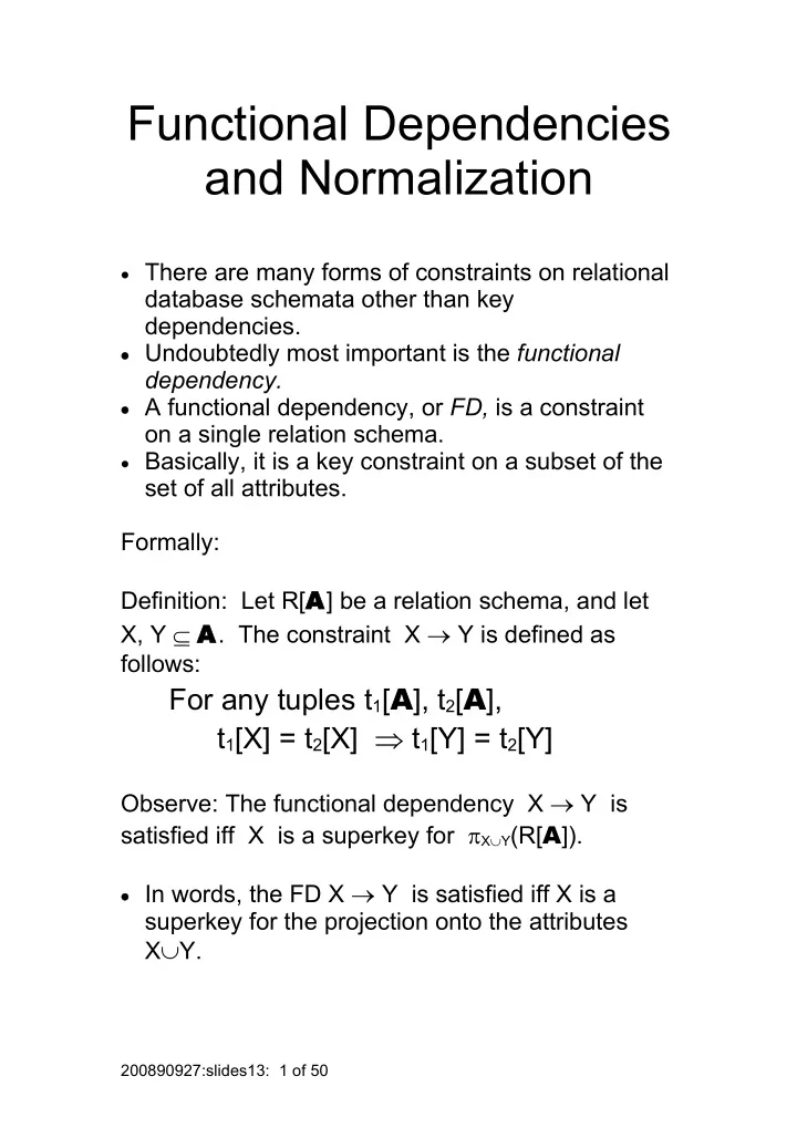
Functional Dependencies and Normalization · There are many forms of constraints on relational database schemata other than key dependencies. · Undoubtedly most important is the functional dependency. · A functional dependency, or FD, is a constraint on a single relation schema. · Basically, it is a key constraint on a subset of the set of all attributes. Formally: Definition: Let R[ A ] be a relation schema, and let X, Y  A . The constraint X  Y is defined as follows: For any tuples t 1 [ A ], t 2 [ A ], t 1 [X] = t 2 [X]  t 1 [Y] = t 2 [Y] Observe: The functional dependency X  Y is satisfied iff X is a superkey for  X  Y (R[ A ]). · In words, the FD X  Y is satisfied iff X is a superkey for the projection onto the attributes X  Y. 200890927:slides13: 1 of 50

Example: Rail_Schedule Engineer Train Date Departure Platform {Train}  { Departure } {Engineer, Date, Departure}  {Train} {Train, Date}  {Engineer, Platform} 200890927:slides13: 2 of 50

Semantic Consequence: It is often the case that if certain FDs hold, then others must hold as well. Examples: If { Train, Date }  { Engineer, Platform } and {Engineer, Date, Departure}  {Train} hold then so does {Engineer, Date, Departure}  { Platform}. If { Train }  { Departure} holds then so does { Train, Engineer }  { Departure}. Formally, let A be a set of attributes, and let F 1 , F 2 , .., F n, and G be FDs over A . G is a semantic consequence of {F 1 , F 2 , .., F n }, written {F 1 , F 2 , .., F n }  G if the FD G holds whenever all of the elements of {F 1 , F 2 , .., F n } do. (This applies to any relation whatever on the attribute set A .) If {G 1 , G 2 , .., G m } is a set of FDs, then {F 1 , F 2 , .., F n }  {G 1 , G 2 , .., G m } means that {F 1 , F 2 , .., F n }  G I for each i, 1  i  m. 200890927:slides13: 3 of 50

Examples: {{Train, Date}  {Engineer, Platform} {Engineer, Date, Departure}  {Train}}  {Engineer, Date, Departure}  {Platform} {{ Train }  Departure}}  {Train, Engineer}  {Departure}. Closure: The set G of all FDs for which {F 1 , F 2 , .., F n }  G holds is called the (semantic) closure of {F 1 , F 2 , .., F n }, and is denoted {F 1 , F 2 , .., F n } + . Two sets of FDs F and G are said to be equivalent if F + = G + . Exterior: The set G of all FDs for which {F 1 , F 2 , .., F n }  G does not hold, written {F 1 , F 2 , .., F n }  / G is called the (semantic) exterior of {F 1 , F 2 , .., F n }, and is denoted {F 1 , F 2 , .., F n }  . Example: {{ Train }  { Departure } {Engineer, Date, Departure}  {Train} {Train, Date}  {Engineer, Platform} }  / {Departure}  {Train}. 200890927:slides13: 4 of 50

Question: How is the relation  determined? · Purely semantic approaches are possible, but impractical. (Compare truth tables in propositional logic.) · Syntactic inference system: A syntactic inference system is a collection of rules which allows us to conclude new assertions ( i.e., FDs) from existing ones. Example: FDs obey a transitive rule. If A  B and B  C both hold (for any attributes A, B , and C whatever), then so too does A  C . Thus, we might include such a rule in a syntactic system. For an inference system, the symbol which is typically used is  . Thus, {F 1 , F 2 , .., F n }  G means that G can be deduced from {F 1 , F 2 , .., F n } by application of the extant system of syntactic rules. (Alternately, there is a proof of G from {F 1 , F 2 , .., F n }.) Example: A possible rule is { A  B, B  C}  A  C. 200890927:slides13: 5 of 50

A Syntactic Proof System: In the following rules, let A be a set of attributes, and let W, X, Y, and Z be arbitrary subsets of A . A1 (Reflexivity): { Y  X }  X  Y. A2 (Augmentation): { X  Y }  X  Z  Y  Z. A3 (Additivity) : { X  Y, X  Z }  X  Y  Z. A4 (Projectivity): { X  Y  Z }  X  Y. A5 (Transitivity): { X  Y, Y  Z }  X  Z. A6 (Pseudotransitivity): { X  Y, Y  Z  W }  X  Z  W. Contrary to the assertion in the text, we cannot “prove” these rules. However, it can be established that they have certain fundamental logical properties. But first, we must be clear about what is meant by an inference. 200890927:slides13: 6 of 50

Definition: Let  be an inference relation, and let  1 ,  2 , ...,  n , and  be assertions. A proof of  from {  1 ,  2 , ...,  n } is a sequence of assertions  1,  2 , ..,  i,  i+1 , ..,  k-1,  k with the property that 1. The final element in the list is the conclusion which is sought; i.e.,  k =  . 2. Every element in the list is either one of the  I ’s or else a consequence, via  , of some of the preceding elements in the list. Formally, for each i, 1  i  k, either  i  {  1 ,  2 , ...,  n } or else    i for some   {  1,  2 , ..,  i-1 }. 200890927:slides13: 7 of 50

Example: Prove {Engineer, Date, Departure}  {Platform} from the axioms of the earlier example. 1. {Train}  {Departure} (Given) 2. {Engineer, Date, Departure}  {Train} (Given) 3. {Train, Date}  {Engineer, Platform} (Given) 4. {Engineer, Date, Departure}  {Train, Date} (A2: Augmentation of 2) 5. {Engineer, Date, Departure}  {Engineer, Platform} (A5: Transitivity on 4 and 3) 6. {Engineer, Date, Departure}  {Platform}. (A4: Projectivity on 5) 200890927:slides13: 8 of 50

Formal properties of inference systems: · Soundness: Everything which can be proven is true. Formally, If { 1 ,  2 , ...,  n }   , then { 1 ,  2 , ...,  n }   . · Completeness: Everything which is true can be proven. Formally, if { 1 ,  2 , ...,  n }   , then { 1 ,  2 , ...,  n }  . · Decidability : There is an algorithm which can apply the proof rules and determine whether or not there is a proof of the desired conclusion from the axioms. (The process cannot loop forever in a search.) Fact: The axioms A1-A6 are sound and complete, and possess a decidable inference algorithm. (It is easy to see that things are decidable in this context. Why?) Fact: The subset consisting of just A1 (Reflexivity), A2 (Augmentation), and A6 (Pseudotransitivity) is complete. 200890927:slides13: 9 of 50

A more intuitive inference system for FDs: The following system is based upon directed acyclic graphs (DAG): · Reduce all FDs to those with only one attribute on the right-hand side (RHS). Example: { Train, Date }  { Engineer, Platform } becomes: {Train, Date}  {Engineer} {Train, Date}  { Platform} Clearly, these two FDs are equivalent to the one above. Call such an FD simple. · Represent each simple FD by a DAG in which the nodes are attributes and the edges run from left- hand side (LHS) attributes to right-hand side (RHS) attributes. Example: The FD { Train, Date}  {Engineer } is represented as follows. Train Engineer Date 200890927:slides13: 10 of 50

Derivations are represented by gluing these graphs together. For example, here is a derivation of {Engineer, Date, Departure}  {Platform}. Engineer Train Departure Platform Date This graph embodies the FDs {Engineer, Date, Departure}  {Train} {Train, Date}  {Platform} as axioms. It derives the FD {Engineer, Date, Departure}  {Platform} because · The LHS attributes are the initial nodes of the graph. · All RHS attributes are named in nodes which are connected to these initial nodes. Fact: This DAG procedure is sound and complete for inference on FDs. (D. Maier, The Theory of Relational Databases, Computer Science Press, 1983.) 200890927:slides13: 11 of 50

Normalization: · Schemata constrained by arbitrary sets of FDs have certain anomalies which make them undesirable. To remedy this situation, there have been quite a number of normal forms proposed which deal with these issues. · There are two approaches to normalization: · In the decomposition approach , one starts with a relational database schema with perhaps only one or a very few relations, and decomposes the relations (using projection) into smaller ones in an effort to remove the problems. · In the synthetic approach , one starts with a set of FDs, and then attempts to construct a relational database schema which embodies those FDs while avoiding any anomalies. · Each approach as its advantages and disadvantages. · Both approaches will be examined in these slides. · First, we need to consider some normal forms. 200890927:slides13: 12 of 50

Normal Forms: · In early papers, E. F. Codd, who is credited with “inventing” the relational model, introduced three normal forms. First Normal Form: This just says that domains consist of atomic values, and may not themselves be structured. In most modern work, this property is built into the model. 200890927:slides13: 13 of 50