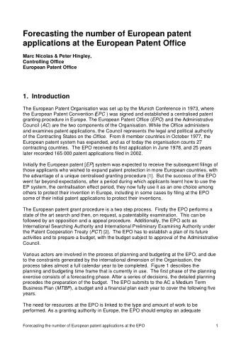
Forecasting Patent Filings at the European Patent Office (EPO) using - PowerPoint PPT Presentation

Forecasting Patent Filings at the European Patent Office (EPO) using compositional data analysis techniques. Peter Hingley, Financial Controlling and Statistics, European Patent Office, M unich, Germany phingley@epo.org Disclaimer: The forecasts that will be mentioned are not official forecasts of EPO. CoDaWork 2017 Workshop Abbadia San Salvatore 8th June 2017

Contents • 1. Patenting at EPO and the forecasting problem. • 2. A Dynamic Log Linear (DLL) model for Total (patent) Filings (TFs). • 3. Fitting the DLL model to TFs. • 4. Fitting a straight line ilr regression model to Industrial Areas (IA) proportions. • 5. Fitting a straight line ilr regression model for TFs with IA proportions as added predictors. • 6. Conclusions

1. Patenting at EPO and the forecasting problem. Patentability under the European Patent Convention (EPC) Patents are granted for inventions in all fields of technology To be patentable, inventions must be new , involve an inventive step and be industrially applicable They must relate to a product, process, apparatus or use. Some things are excluded from patentability (E.G. Discoveries; Scientific theories, Mathematical methods, Computer programs, ....) Patents are an incentive for economic growth. § Makes the latest technological knowledge available to the public § Inspires further innovation § Helps to prevent duplication of R&D § Helps identify new partners and allows licensing § Gives patent holders time to recoup their development costs 3 European Patent Office

1. Patenting at EPO and the forecasting problem. Total Filings (TFs) are the sums of these areas. First filing Subsequent filing within 12 months First filing + 30 months 1) By claiming priority of an earlier application filed with a national office (or at WIPO) within 12 months. First filings (Euro-PCT-INT) can also be done at EPO but numbers are small enough to ignore. 4 European Patent Office

1. Patenting at EPO and the forecasting problem. There are various ways to classify patents by technical areas. The International Patent Classification (IPC) system is well established. IPC has 8 main classes (A to H) and many sub-classes. IPC assignment is by technical content. Assigning to industries of applicants is also possible. 5 European Patent Office

1. Patenting at EPO and the forecasting problem. CODA approach to relationships between IPC proportions. Principal components (or regressions) could be useful for technical trends in patent applications. But this does not solve the forecasting problem for T otal Filings (TFs) at EPO. European Patent Office 6

1. Patenting at EPO and the forecasting problem. Breaking down TFs into just three Industrial Areas (IAs), Electricals , Chemicals and Traditionals is more manageable for forecasting purposes. The numbers of Filings with no IA assigned increases after 2013. 2–way breakdowns (Blocs vs IAs) are not considered advisable.

2. A Dynamic Log Linear (DLL) model for EPO Total filings for patents (TFs). Dynamic log linear models Country of origin breakdowns are built Country 1 Country 2 Autoregre- Factor in. Intercept Intercept ssive terms B 1 0 - - COUNTRY 1 A 1 0 - - 1 0 - - B DIVIDE BY POPULATION 1 0 - - SIZE OF COUNTRY, 1 0 - - TAKE LOGARITHMS 1 0 - - 0 1 - - 0 1 - - COUNTRY 2 A 0 1 - - 0 1 - - B 0 1 - - DESIGN MATRIX X Time . Linear Model for filings A: Y = X . B B = (X T X) -1 . X T Y . Estimate . Fit & Forecast Y = X . B Back transform per country, add filings estimates per year Series A: Filings to be forecast Series B, C ...: Explanatory variables 8

2. A Dynamic Log Linear (DLL) model for EPO Total filings for patents (TFs). An approach including the Influence of Business Cycles. where P is the number of EPO T otal filings from a country; L is the number of workers in a country; i is the country; t is time (years); -1 and -2 indicate lags of one year or two years; R is R&D expenditures - a stock variable with components from 0 to 5 year lags; The GDP of the source country Y is split into two components:- T is the “ trend” level of output Y u is the business cycle variable; α terms are estimable parameters ( α i is a country intercept); ε it is an error term, assumed to be normal with constant variance; ln( ) denotes natural logarithm; and ∆ indicates year-to-year differences. European Patent Office 9

2. A Dynamic Log Linear (DLL) model for EPO Total filings for patents (TFs). Include two Isometric Log-Ratio (ilr) terms to a cut-down version of the DLL model. Fit two ilr terms rather than three to avoid collinearity. Training data run from year 2001 up to year 2015. M odels fitted up to end of calendar year two years before. So in January 2017, the model was fitted up to 2015. European Patent Office 10

3. Fitting the DLL model to TFs. Parameter estimates after fitting the various models. * indicates approximate significance at the 95 percent level. Separate Industrial Areas (IAs) Total Filings Parameter estimates Electricity (E) Chemistry (C) Traditional (T) With IAs Without IAs α 2 Autoregression -0.01 -0.18* -0.05 -0.09* -0.08* α 3 R&D Stock 0.29 0.27 0.09 0.36* 0.36* α 4 GDP trend -0.25 2.51* 1.63* 1.26* 1.12* α 5 GDP cycle 0.39 0.2 0.44 0.53 0.46 α 6 ilr for Electricals 0.30* α 7 ilr for Chemicals 0.21* Observation standard error 0.1877 0.1653 0.1325 0.111 0.113 Residual degrees of freedom 388 388 388 386 388 M odel with IAs fits No Significant Significant α 2 & α 4 α 4 better than w/ o IAs. significant parameters. parameters. parameter.

3. Fitting the DLL model to TFs. Total Filings forecasts, both with and without ilr terms for IAs, are almost exactly the same. (M odel fit is better with ilr terms). These forecasts are lower than cumulating the forecasts by IAs.

4. Fitting a straight line ilr regression model to IA proportions. Forecasts of proportions of IAs in TFs, based on: - Straight line regressions to the raw proportions; Straight line regressions after transforming proportions to ilrs; and Straight line regressions after transforming proportions to ilrs and including TFs as an additional predictor. (Back-transformation of fitted ilrs to proportions was done in Excel.)

4. Fitting a straight line ilr regression model to IA proportions. Back transformation of predicted isometric logratio ( ilr j ) terms to proportions ( p j ). But what is k? Create a column of trial values of k, k 1 say, of sufficient accuracy. Calculate Estimate k by minimising | k1 – k2| . European Patent Office 14

5. Fitting a straight line ilr regression model for TFs with IA proportions as added predictors.

6. Conclusions. 1. When modelling TFs, the fit of the DLL model is improved by adding terms based on IAs. Similarly, a straight line regression for TFs gives improved fit by adding terms based on IAs. BUT In both cases, forecasts of TFs are hardly changed by including the IA terms. 2. When modelling proportions of IAs by straight line regressions of ilr based terms, the results are almost the same as fitting straight lines directly to the proportions. BUT The CoDa approach will work better with many classes or low/ high proportions for some classes. 3. Possible methods have been identified to add a Total to a model of proportions (in straight line regressions of ilrs), or ilr proportions to models for the total (in DLL model and straight line regressions). BUT Here, so far, forecasts are hardly changed although model fits improve. European Patent Office 16

6. Conclusions. 4. Theoretical modelling including simulations could better resolve issues raised under point 3. Perhaps an iterative approach can model both Totals and proportions simultaneously. 5. A suggestion to use a “Total” that relates to a geometric mean could be explored using analysis as at point 4. This could further improve the agreement of forecasts with and without additional terms. Any remaining discrepancy could be due to the approximation of modelling a total from the geometric mean. 6. Extensions of the CoDa approach to modelling patent filings (Totals and/ or proportions) could investigate other breakdowns, like first/ subsequent filings and patent families. THANK YOU European Patent Office 17