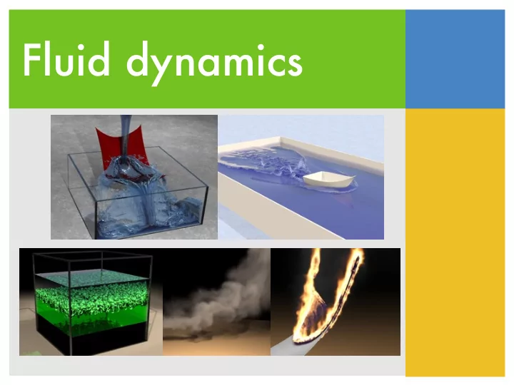
Fluid dynamics Math background Physics Simulation Related - PowerPoint PPT Presentation

Fluid dynamics

• Math background • Physics • Simulation • Related phenomena • Frontiers in graphics • Rigid fluids

Fields • Domain Ω ⊆ R 2 • Scalar field f : Ω → R • Vector field f : Ω → R 2

Types of derivatives • Derivatives measure how something changes due to its parameters ∂f • Temporal derivatives ∂t • Spatial derivatives � T � ∂f ∂x, ∂f • gradient operator ∇ f = ∂y ∇ · f = ∂ f x ∂x + ∂ f y • divergence operator ∂y ∇ 2 f = ∇ · ( ∇ f ) = ∂ 2 f ∂x + ∂ 2 f • Laplacian operator ∂y

• Math background • Physics • Simulation • Related phenomena • Frontiers in graphics • Rigid fluids

Representation Density ρ : Ω → [0 , 1] Domain Ω Velocity u : Ω → R 3

“Coffee cup” equation Navier-Stokes Momentum ∂t = − ( u · ∇ ) u − 1 ∂ u ρ ∇ p + s ∇ 2 u + f equation Incompressibility u : velocity ∇ · u = 0 condition p : pressure s : kinematic viscosity f : body force ρ : fluid density

Momentum equation • Each particle represents a little blob of fluid with mass m , a volume V , and a velocity u • The acceleration of the particle a ≡ D u Dt • The Newton’s law mD u Dt = F

Forces acting on fluids • Gravity: m g • Pressure: - ∇ p • Imbalance of higher pressure • Viscosity: µ ∇ · ∇ u • Force that makes particle moves at average speed • dynamic viscosity coefficient: µ

Momentum equation The movement of a blob of fluid mD u Dt = m g − V ∇ p + V µ ∇ · ∇ u Divide by volume ρD u Dt = ρ g − ∇ p + µ ∇ · ∇ u Rearrange equation giving Navier-Stoke D u Dt + 1 ρ ∇ p = g + s ∇ · ∇ u

Lagrangian v.s. Eulerian • Lagrangian point of view describes motion as points travel around space over time • Eulerian point of view describes motion as the change of velocity field in a stationary domain • Lagrangian approach is conceptually easier, but Eulerian approach makes the spatial gradient easier to compute/approximate

Material derivative Dq Dt = ∂q ∂t + u ∂q ∂x + v ∂q ∂y + w ∂q ∂z dtq ( t, x ) = ∂ q d ∂ t + ∇ q · d x dt = ∂ q ∂ t + ∇ q · u = Dq Dt

Advection • Advection describe how quantity, q , moves with the velocity field u • Density Dρ Dt = ∂ρ ∂t + u · ∇ ρ • Velocity Dt = ∂ u D u ∂ t + u · ∇ u

Advection momentum D u Dt + 1 ρ ∇ p = g + s ∇ · ∇ u equation Advection Projection Diffusion Body force ∂t = − ( u · ∇ ) u − 1 ∂ u ρ ∇ p + s ∇ 2 u + f ∇ · u = 0

Density advection ∂ρ ∂ t = − ( u · ∇ ) ρ

Velocity advection ∂ t = − ( u · ∇ ) u − 1 ∂ u ρ ∇ p + s ∇ 2 u + f s.t. ∇ · u = 0

Projection Advection Projection Diffusion Body force ∂t = − ( u · ∇ ) u − 1 ∂ u ρ ∇ p + s ∇ 2 u + f ∇ · u = 0

Divergence free ∇ · u > 0? ∇ · u < 0?

Divergence free ∇ ∙ u = 0 ∇ ∙ u ≠ 0

Projection ∂ t = − ( u · ∇ ) u − 1 ∂ u ρ ∇ p + s ∇ 2 u + f s.t. ∇ · u = 0

Diffusion Advection Projection Diffusion Body force ∂t = − ( u · ∇ ) u − 1 ∂ u ρ ∇ p + s ∇ 2 u + f ∇ · u = 0

High viscosity fluids

Dropping viscosity • Viscosity plays a minor role in most fluids • Numeric methods introduce errors which can be physically reinterpreted as viscosity • Fluid with no viscosity is called “inviscid”

Body force Advection Projection Diffusion Body force ∂t = − ( u · ∇ ) u − 1 ∂ u ρ ∇ p + s ∇ 2 u + f ∇ · u = 0

External forces • Gravity • Heat • Surface tension • User-specified forces (stirring coffee)

Boundary conditions • Solid walls • The fluid cannot go in and out of it • Control the normal velocity • Free surfaces • Air can be represented as a region where the pressure is zero • Do not control the velocity at the surface

Solid boundary • Velocity at the boundary u · ˆ n = u solid · ˆ n • No-slip condition: u = u solid • Pressure at the boundary • Make the fluid incompressible AND enforce the solid boundary condition

Physics recap • Physical quantity represented as fields • Navier-Stokes PDE describes the dynamics

• Math background • Physics • Simulation • Related phenomena • Frontiers in graphics • Rigid fluids

Challenges • What is the representation for fluids? • represent velocity and pressure • What is the equation of motion for fluids? • approximate Navier-Stokes in a discrete domain • compute Navier-Stokes efficiently

Grid structure p i,j +1 v i,j +1 / 2 p i +1 ,j p i − 1 ,j p i,j u i − 1 / 2 ,j u i +1 / 2 ,j v i,j − 1 / 2 p i,j − 1

Explicit integration • Solving for the differential equation explicitly, namely ∂t = − ( u · ∇ ) u − 1 ∂ u ρ ∇ p + s ∇ 2 u + f u t +1 = u t + h ˙ u ( t ) • You get this...

Explicit integration

Stable fluids Invented by Jos Stam Simple, fast, and unconditionally stable

Splitting methods • Suppose we had a system ∂x ∂t = f ( x ) = g ( x ) + h ( x ) • We define simulation function S f S f ( x, ∆ t ) : x ( t ) → x ( t ) + ∆ tf ( x ) • Then we could define S f ( x, ∆ t ) : x ( t + ∆ t ) = S g ( x, ∆ t ) ◦ S h ( x, ∆ t )

Splitting methods ∂t = − ( u · ∇ ) u − 1 ∂ u ρ ∇ p + s ∇ 2 u + f w 0 = u ( x , t ) add force Advect Diffuse Project w 0 ( x ) w 1 ( x ) w 2 ( x ) w 3 ( x ) w 4 ( x ) u ( x , t + Δ t ) = w 4

Splitting methods ∂t = − ( u · ∇ ) u − 1 ∂ u ρ ∇ p + s ∇ 2 u + f w 0 = u ( x , t ) add force Advect Diffuse Project w 0 ( x ) w 1 ( x ) w 2 ( x ) w 3 ( x ) w 4 ( x ) u ( x , t + Δ t ) = w 4

Body forces

Splitting methods ∂t = − ( u · ∇ ) u − 1 ∂ u ρ ∇ p + s ∇ 2 u + f w 0 = u ( x , t ) add force Advect Diffuse Project w 0 ( x ) w 1 ( x ) w 2 ( x ) w 3 ( x ) w 4 ( x ) u ( x , t + Δ t ) = w 4

Advection

Numerical dissipation • Semi-Lagrangian advection tend to smooth out sharp features by averaging the velocity field • The numerical errors result in a different advection equation solved by semi-Largrangian ∂ x = u ∆ x ∂ 2 q ∂ q ∂ t + u ∂ q ∂ x 2 • Smooth out small vortices in inviscid fluids

Splitting methods ∂t = − ( u · ∇ ) u − 1 ∂ u ρ ∇ p + s ∇ 2 u + f w 0 = u ( x , t ) add force Advect Diffuse Project w 0 ( x ) w 1 ( x ) w 2 ( x ) w 3 ( x ) w 4 ( x ) u ( x , t + Δ t ) = w 4

Diffusion • Solve for the effect of viscosity ∂ w 2 = ν ∇ 2 w 2 ∂ t • Use an implicit method for stable result ( I − ν ∆ t ∇ 2 ) w 3 ( x ) = w 2 ( x )

Splitting methods ∂t = − ( u · ∇ ) u − 1 ∂ u ρ ∇ p + s ∇ 2 u + f w 0 = u ( x , t ) add force Advect Diffuse Project w 0 ( x ) w 1 ( x ) w 2 ( x ) w 3 ( x ) w 4 ( x ) u ( x , t + Δ t ) = w 4

Projection P( )

Projection • Projection step subtracts off the pressure from the intermediate velocity field w 3 w 4 = w 3 − ∆ t 1 ρ ∇ p • project ( Δ t, u ) must satisfies two conditions: ∇ · u t +1 = 0 • divergence free: • boundary velocity: u t +1 · ˆ n = u solid · ˆ n

Boundary conditions • Dirichlet boundary condition for free surfaces • Neumann boundary condition for solid walls i +1 / 2 ,j = u i +1 / 2 ,j − ∆ t 1 p i +1 ,j − p i,j u t +1 ∆ x ρ p i,j p i +1 ,j since u t +1 i +1 / 2 ,j = u solid u i +1 / 2 ,j p i +1 ,j = p i,j + ρ ∆ x ∆ t ( u i +1 / 2 ,j − u solid )

Divergence-free condition p i,j +1 u t +1 i +1 / 2 ,j − u t +1 v t +1 i,j +1 / 2 − v t +1 i − 1 / 2 ,j i,j − 1 / 2 + = 0 ∆ x ∆ x v i,j +1 / 2 replace u t +1 i +1 / 2 ,j (and other terms) p i +1 ,j p i − 1 ,j p i,j u i − 1 / 2 ,j u i +1 / 2 ,j u i +1 / 2 ,j − ∆ t 1 p i +1 ,j − p i,j with v i,j − 1 / 2 ∆ x ρ p i,j − 1 result in a discrete Poisson equation � 4 p i,j − p i +1 ,j − p i,j +1 − p i − 1 ,j − p i,j − 1 � � u i +1 / 2 ,j − u i − 1 / 2 ,j � ∆ t + v i,j +1 / 2 − v i,j − 1 / 2 = − ∆ x 2 ∆ x ∆ x ρ

The pressure equations p i,j +1 • If grid cell (i, j + 1) is in air and (i+1, j) is a solid v i,j +1 / 2 p i +1 ,j • replace p i , j +1 with zero p i − 1 ,j p i,j u i − 1 / 2 ,j u i +1 / 2 ,j • replace p i+ 1, j with the value v i,j − 1 / 2 from Neumann condition p i,j − 1 p i,j + ρ ∆ x ∆ t ( u i +1 / 2 ,j − u solid ) 0 � 4 p i,j − p i +1 ,j − p i,j +1 − p i − 1 ,j − p i,j − 1 � � u i +1 / 2 ,j − u i − 1 / 2 ,j � ∆ t + v i,j +1 / 2 − v i,j − 1 / 2 = − ∆ x 2 ∆ x ∆ x ρ

Solve a linear system • Ap = b • Construct matrix A : • diagonal entry: # of non-solid neighbors • off-diagonal: 0 if the neighbor is non-fluid cell and -1 if the neighbor is fluid cell • A is symmetric positive definite • Use preconditioned conjugate gradient