flow Solve pixel correspondence problem given a pixel in H, look - - PDF document

1

Announcements

• Quiz Thursday
• Quiz Review Tomorrow: AV Williams 4424,

4pm.

• Practice Quiz handout.

Matching

• Compare region of image to region of image.

– We talked about this for stereo. – Important for motion.

• Epipolar constraint unknown.
• But motion small.

– Recognition

• Find object in image.
• Recognize object.
• Today, simplest kind of matching. Intensities

similar.

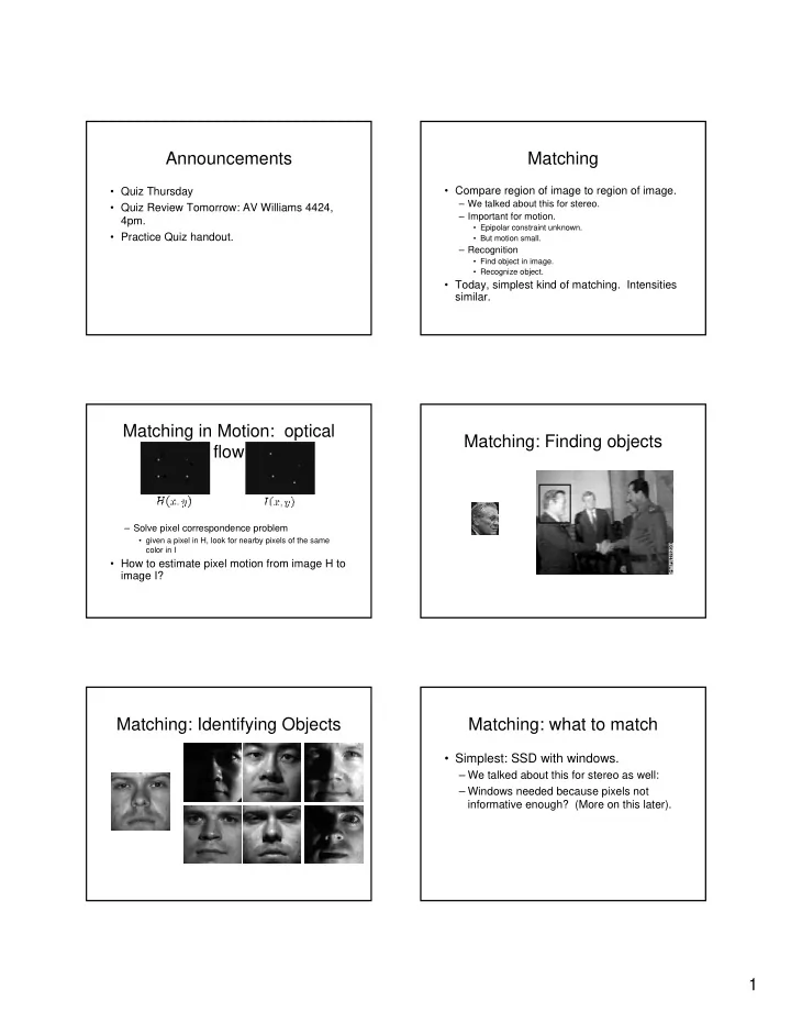
Matching in Motion: optical flow

• How to estimate pixel motion from image H to

image I?

– Solve pixel correspondence problem

• given a pixel in H, look for nearby pixels of the same

color in I

Matching: Finding objects Matching: Identifying Objects Matching: what to match

• Simplest: SSD with windows.

– We talked about this for stereo as well: – Windows needed because pixels not informative enough? (More on this later).

2

Comparing Windows:

= ? f g Most popular (Camps)

Window size

W = 3 W = 20 Better results with adaptive window

• T. Kanade and M. Okutomi, A Stereo Matching

Algorithm with an Adaptive Window: Theory and Experiment,, Proc. International Conference on Robotics and Automation, 1991.

• D. Scharstein and R. Szeliski. Stereo matching with

nonlinear diffusion. International Journal of Computer Vision, 28(2):155-174, July 1998

• Effect of window

size (Seitz)

Subpixel SSD

• When motion is a few pixels or less,

motion of an integer no. of pixels can be insufficient.

Bilinear Interpolation

To compare pixels that are not at integer grid points, we resample the image. Assume image is locally bilinear. I(x,y) = ax + by + cxy + d = 0. Given the value of the image at four points: I(x,y), I(x+1,y), I(x,y+1), I(x+1,y+1) we can solve for a,b,c,d linearly. Then, for any u between x and x+1, for any v between y and y+1, we use this equation to find I(u,v).

Matching: How to Match Efficiently

• Baseline approach: try everything.

– Could range over whole image. – Or only over a small displacement.

( )

∑

+ + −

2 ,

) , ( ) , ( min arg v y u x I y x W

v u

search search search search

Matching: Multiscale

(Weizmann Institute Vision Class)

3

2 ) * (

2 3

↓ = gaussian G G

1

G

3

G

The Gaussian Pyramid

High resolution Low resolution Image = G 2 ) * (

1

↓ = gaussian G G 2 ) * (

1 2

↓ = gaussian G G 2 ) * (

3 4

↓ = gaussian G G blur blur blur down-sample down-sample d

• w

n

• s

a m p l e

2

G

4

G blur down-sample (Weizmann Institute Vision Class)

When motion is small: Optical Flow

• Small motion: (u and v are less than 1 pixel)
• Brute force not possible
• suppose we take the Taylor series expansion of I:

(Seitz)

Optical flow equation

• Combining these two equations
• In the limit as u and v go to zero, this

becomes exact

(Seitz)

Optical flow equation

• Q: how many unknowns and equations per

pixel?

• Intuitively, what does this constraint

mean?

– The component of the flow in the gradient direction is determined – The component of the flow parallel to an edge is unknown

This explains the Barber Pole illusion http://www.sandlotscience.com/Ambiguous/barberpole.htm

(Seitz)

First Order Approximation

When we assume that: We assume an image locally is: (Seitz)

Aperture problem

(Seitz)

4

Aperture problem

(Seitz)

Solving the aperture problem

• How to get more equations for a pixel?

– Basic idea: impose additional constraints

• most common is to assume that the flow field is smooth

locally

• one method: pretend the pixel’s neighbors have the

same (u,v)

– If we use a 5x5 window, that gives us 25 equations per pixel!

(Seitz)

Lukas-Kanade flow

• We have more equations than unknowns: solve least

squares problem. This is given by:

– Summations over all pixels in the KxK window – Does look familiar?

(Seitz)

Conditions for solvability

– Optimal (u, v) satisfies Lucas-Kanade equation

When is This Solvable?

• ATA should be invertible
• ATA should not be too small due to noise

– eigenvalues λ1 and λ2 of ATA should not be too small

• ATA should be well-conditioned

– λ1/ λ2 should not be too large (λ1 = larger eigenvalue) (Seitz)

Does this seem familiar? Formula for Finding Corners

        =

∑ ∑ ∑ ∑

2 2 y y x y x x

I I I I I I C

We look at matrix:

Sum over a small region, the hypothetical corner Gradient with respect to x, times gradient with respect to y Matrix is symmetric

WHY THIS?

      =         =

∑ ∑ ∑ ∑

2 1 2 2

λ λ

y y x y x x

I I I I I I C

First, consider case where:

This means all gradients in neighborhood are: (k,0) or (0, c) or (0, 0) (or off-diagonals cancel). What is region like if:

• 1. λ1 = 0?
• 2. λ2 = 0?
• 3. λ1 = 0 and λ2 = 0?
• 4. λ1 > 0 and λ2 > 0?

5

General Case:

From Singular Value Decomposition it follows that since C is symmetric:

R R C       =

− 2 1 1

λ λ

where R is a rotation matrix. So every case is like one on last slide.

So, corners are the things we can track

• Corners are when λ1, λ2 are big; this is

also when Lucas-Kanade works.

• Corners are regions with two different

directions of gradient (at least).

• Aperture problem disappears at

corners.

• At corners, 1st order approximation fails.

Edge

– large gradients, all the same

– large λ1, small λ2

(Seitz)

Low texture region

– gradients have small magnitude

– small λ1, small λ2

(Seitz)

High textured region

– gradients are different, large magnitudes

– large λ1, large λ2

(Seitz)

Observation

• This is a two image problem BUT

– Can measure sensitivity by just looking at one of the images! – This tells us which pixels are easy to track, which are hard

• very useful later on when we do feature tracking...

(Seitz)

6

Errors in Lukas-Kanade

• What are the potential causes of errors in this

procedure?

– Suppose ATA is easily invertible – Suppose there is not much noise in the image

• When our assumptions are violated

– Brightness constancy is not satisfied – The motion is not small – A point does not move like its neighbors

• window size is too large
• what is the ideal window size?

(Seitz)

Iterative Refinement

• Iterative Lukas-Kanade Algorithm
• 1. Estimate velocity at each pixel by solving Lucas-

Kanade equations

• 2. Warp H towards I using the estimated flow field
• use bilinear interpolation
• Repeat until convergence

(Seitz)

If Motion Larger: Reduce the resolution

(Seitz)

Optical flow result

Dewey morph

(Seitz)

Tracking features over many Frames

• Compute optical flow for that feature for each

consecutive H, I

• When will this go wrong?

– Occlusions—feature may disappear

• need to delete, add new features

– Changes in shape, orientation

• allow the feature to deform

– Changes in color – Large motions

• will pyramid techniques work for feature

tracking? (Seitz)

Applications:

• MPEG—application of feature tracking

– http://www.pixeltools.com/pixweb2.html

(Seitz)

7

Image alignment

• Goal: estimate

single (u,v) translation for entire image – Easier subcase: solvable by pyramid-based Lukas-Kanade (Seitz)

Summary

• Matching: find translation of region to

minimize SSD.

– Works well for small motion. – Works pretty well for recognition sometimes.

• Need good algorithms.

– Brute force. – Lucas-Kanade for small motion. – Multiscale.

• Aperture problem: solve using corners.

– Other solutions use normal flow.

This document was created with Win2PDF available at http://www.daneprairie.com. The unregistered version of Win2PDF is for evaluation or non-commercial use only.