flour beetles, Tribolium castanium thanks: science.nayland.school.nz - - PowerPoint PPT Presentation

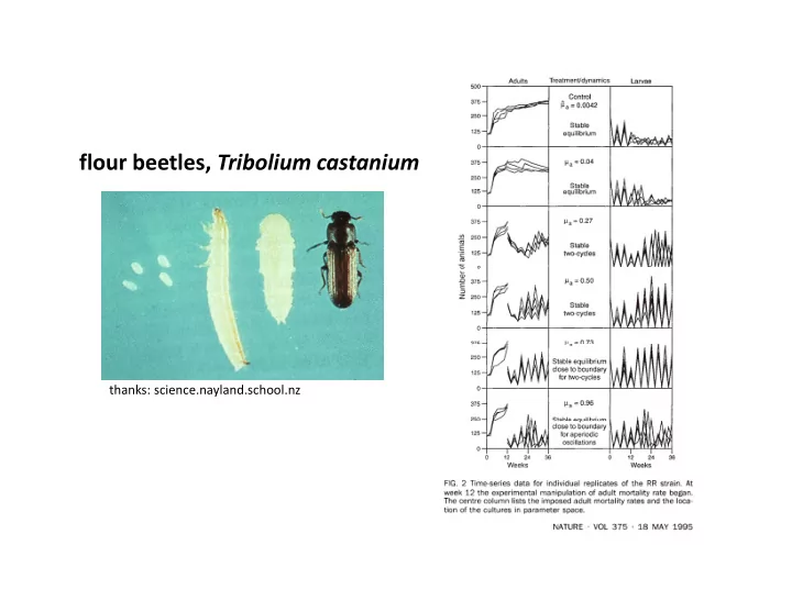
flour beetles, Tribolium castanium

thanks: science.nayland.school.nz

Some important distinctions Cohort life table: Follow the fate of a group of individuals all born during the same time interval (a k a longitudinal born during the same time interval. (a.k.a. longitudinal data) Segment life table: Follow all individuals alive during the same time interval. (a.k.a. static life table)

Some important distinctions Birth‐flow: Births occur continually Birth‐pulse: Births occur once per time step, and at a common point in time. For birth‐pulse populations, we further distinguish between: pre‐breeding census: births occur immediately after parents graduate to a new age class post‐breeding census: births occur immediately before parents graduate to a new age class

Definitions and notation S( ) F h lif bl h b f i di id l h S(x): For a cohort life table, the number of individuals that survive to age x. S(0): Initial size of cohort. k: Age by which all individuals have died k: Age by which all individuals have died. Survivorship, l(x): Fraction of cohort that survives to age x (i l i i l) (i.e., cumulative survival) ( ) ( ) (0) S x l x S  Survival rate, g(x): Fraction of cohort alive at age x that survives to age x+1 (0) S ( 1) S survives to age x+1. ( 1) ( ) ( ) S x g x S x  

Definitions and notation Survivorship can also be defined in terms of survival rate: ( ) (0) (1) ( 1) l x g g g x       Some authorities (but not Populus) define the mortality rate as ( ) 1 ( ) m x g x   Fecundity, b(x) (alt. maternity, m(x)): The average number ( ) 1 ( ) m x g x 

• f female offspring born per unit time to an individual

female parent of age x.

Calculations (assuming a post‐breeding, birth‐pulse population) Survivorship, l(x), and fecundity, b(x), schedules yield: net reproductive rate, R0: average number of female

• ffspring produced per female parent over her lifetime

k

generation time G: average age of the parents of all ( ) ( )

k x

R l x b x



 generation time, G: average age of the parents of all

• ffspring (at the time of their births) produced by a single

cohort.

k

( ) ( )

k x

l x b x x G R



  R

x S(x) b(x) l(x) g(x) 100 1 90 1 90 2 80 1 3 40 3 4

x S(x) b(x) l(x) g(x) 100 1 0.9 1 90 0 9 0 89 1 90 0.9 0.89 2 80 1 0.8 0.5 3 40 3 0.4 4

Calculations (assuming a post‐breeding, birth‐pulse population) Survivorship, l(x), and fecundity, b(x), schedules yield: instantaneous rate of population increase, r, or population multiplication rate, . Same as before. Given “implicity” by the Euler equation: by the uler equation: 1 ( ) ( )

k rx x

e l x b x

 

 1 ( ) ( )

k x x

l x b x

 

