
SLIDE 1
Fixing the Blackbody Problem
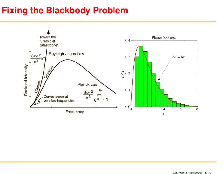
Ε hΝ 2 4 6 8 0.0 0.1 0.2 0.3 0.4 Ε Ε PΕ Planck’s Guess
Experimental Foundations – p. 1/7
Fixing the Blackbody Problem Plancks Guess 0.4 0.3 h P 0.2 - - PowerPoint PPT Presentation
Fixing the Blackbody Problem Plancks Guess 0.4 0.3 h P 0.2 0.1 0.0 0 2 4 6 8 Experimental Foundations p. 1/7 Electromagnetic Waves See more and here and here. Experimental Foundations p. 2/7
Ε hΝ 2 4 6 8 0.0 0.1 0.2 0.3 0.4 Ε Ε PΕ Planck’s Guess
Experimental Foundations – p. 1/7
Experimental Foundations – p. 2/7
d
Experimental Foundations – p. 3/7
Experimental Foundations – p. 4/7
Experimental Foundations – p. 5/7
Experimental Foundations – p. 6/7
Experimental Foundations – p. 7/7