Fitting Large-Scale Spatial Models with Applications to Microarray - - PowerPoint PPT Presentation

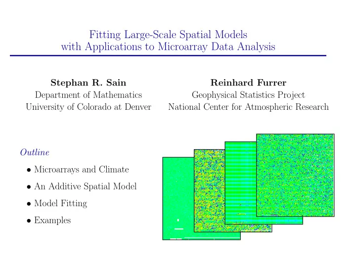
Fitting Large-Scale Spatial Models with Applications to Microarray Data Analysis

Stephan R. Sain Department of Mathematics University of Colorado at Denver Reinhard Furrer Geophysical Statistics Project National Center for Atmospheric Research Outline

• Microarrays and Climate
• An Additive Spatial Model
• Model Fitting
• Examples

Introduction

• Many spatial problems are inherently multivariate – more than one measurement
• r observations at each spatial location.

– Advent of GIS, modern computing, and methodological advances.

• Many spatial problems involve lots of spatial locations.

– Problems in constructing and working with design and covariance matrices.

• Propose a simple multivariate spatial model and discuss some strategies for fitting

and examining the results.

Microarrays and Climate

• Combining observed data and climate models

– Examine model behavior as well as predictions of climate change. – Precipitation and temperature for sixteen models on a 5◦ grid. 2 × 36 × 72 ≈ 5000 observations per chip/model.

• Microarray analysis

– Build a profile of differentially expressed genes relating to cerebral vascular malformations. – Roughly 20 chips with three disease groups (control, AVM, CCM) with each chip a 640 × 640 array 2 × 16 × 12K ≈ 400K observations per chip.

A Multivariate, Additive Spatial Model

• Let Y = [Y′

1 . . . Y′ k]′ where each Yi denotes one spatial variable (one climate

model, one microarray chip, etc.).

• Then,

Y = Xβ + h + ǫ where – Xβ represent fixed effects – h represents a random, zero-mean spatial process – ǫ represents a random error process orthonormal to h.

A Multivariate, Additive Spatial Model

• The structure of X includes both chip specific and gene specific (across chip)

terms: X =      1 R C · · · G 1 R C . . . . . . . . . ... 1 R C G      , where – 1 is a vector of 1s – R and C represent row and column effects – G indicate gene effects.

A Multivariate, Additive Spatial Model

• Further, the model suggests

E[Y] = Xβ Var[Y] = Σh + Σǫ where Σh =      K1 · · · K2 . . . . . . ... Kk      Σǫ =      σ2

1I

· · · σ2

2I

. . . . . . ... σ2

kI

     where – Ki = K(θi) represents a chip specific spatial covariance matrix parameterized by θi – σ2

i are chip specific variances (nugget).

Backfitting

• Ideally, one could use REML to fit covariance parameters and then estimates of

β and predictions of the random effects follow directly: ˆ β = (X′V−1X)−1X′V−1Y (generalized least-squares) ˆ h = ΣhV−1(Y − Xˆ β) where V = Σh + Σǫ

• Direct computation of the design and covariance matrices impractical, not to

mention the matrix computations...

• Quick overview of backfitting from additive models...

Backfitting

• We estimate iteratively the fixed effects and the spatial process.
• Algorithm:

[1] Let h(0) be an inital guess and put j = 1 [2a] β(j) =

• X′X

−1X′ Y − h(j−1) [2b] Estimate covariance parameters, then

• h(j) = ΣhV−1

Y − X β(j) [3] Put j = j + 1 and repeat [2a] and [2b] until convergence

• To prove equivalence at convergence, plug [2b] into [2a].

Straightforward manipulations lead to the generalized least-squares estimator.

• Equivalent to universal kriging.

Backfitting

• Goal: computation in R on a computer with 2 GBytes RAM.
• We perform the regression step iteratively on the chip specific effects and the

gene effects: [2a’]

• β(j)

Chip =

• (1RC)′(1RC)

−1(1RC)′ Y − h(j−1) [2a’’]

• β(j)

Gene =

• G′G

−1G′ Y − h(j−1) [2a’’’] Repeat [2a’] and [2a’’] until convergence

• We need to reconstruct the individual design matrices for each step.
• Calculation time for entire model ≈ 2 minutes per iteration (Xeon i686, Linux).
• Quick convergence: MSE
• β(j) −

β(j−1) < 10−4 for j ≥ 4.

Sparse Matrix Manipulation

• Matrices are stored in a sparse format.
• Design matrix X contains only {0, 1} and Σh has a lot of zeros due to tapering.
• Illustration with “small” sub-design matrix C (Base and SparseM library in R):

Sparse format Full format Sum contr. treatment contr. Storage of C: x Calculate C′C Storage of C′C: x Solve (C′C)x = v: s s s

Covariance Tapering

• Introduce sparseness structure in covariance matrix Ki with some taper function.
• Carefully chosen taper preserves asymptotic optimality with kriging

(Furrer et al. 2004, submitted).

0.0 0.2 0.4 0.6 0.8

Covariance Lag

Exponential (green), spheric (yellow), Tapered = exponential × spheric (red).

• Tapering with range of 2 (eight neighbors):

Nonzero elements in Ki: 3,614,762 (0.002%) Nonzero elements in Cholesky factor of Ki: 67,070,820 (0.040%) With 12 and more neighbors, more than 230 nonzero elements in Cholesky factor.

Microarray Example – A Single Chip

• Few missing values (1.5%).
• Add

blurring to recompense rounding.

• . . .

Microarray Example – A Single Chip

• Estimate the covariance structure.
• Fit an exponential covariance

(range, sill, nugget) = (1.528, 0.487, 0.061).

• Taper with a spherical covariance with range 2.

1 2 3 4 5 6 7 0.0 0.2 0.4 lag

• +

+ + + + + + + x x x x x x x x

+ x empirical horizontal empirical vertical empirical off−axis fitted exponential tapered covariance: exp*spher taper covariance

Microarray Example – A Single Chip

Row/Column effects

100 200 300 400 500 600 −0.2 0.2 Column effects 100 200 300 400 500 600 −0.2 0.2 Row effects

Microarray Example – A Single Chip

Gene effects (normed on the right)

−1 1 2 3 4 −1 1 2 3 4 Perfect match Miss match −5 5 10 15 −5 5 10 15 Perfect match Miss match

Microarray Example – A Single Chip

QQ-plots of gene effects (normed on the right)

−4 −2 2 4 −1 1 2 3 4 Theoretical Quantiles Sample Quantiles 1% 5% 25% 75% 95% 99% −4 −2 2 4 5 10 15 Theoretical Quantiles Sample Quantiles 1% 5% 25% 75% 95% 99%

Microarray Example – A Single Chip

Y = mean + row effects + column effects + spatial process + gene effects + error

Microarray Example – A Single Chip

Y = mean + row effects + column effects + spatial process + gene effects + error

Microarray Example – A Single Chip

Y = mean + row effects + column effects + spatial process + gene effects + error

Microarray Example – A Single Chip

Y = mean + row effects + column effects + spatial process + gene effects + error

Microarray Example – A Single Chip

Y = mean + row effects + column effects + spatial process + gene effects + error

Microarray Example – A Single Chip

Y = mean + row effects + column effects + spatial process + gene effects + error

Microarray Example – A Single Chip

Y = mean + row effects + column effects + spatial process + gene effects + error

Microarray Example – A Single Chip

Y = mean + row effects + column effects + spatial process + gene effects + error

Microarray Example – A Single Chip

Y = mean + row effects + column effects + spatial process + gene effects + error

Microarray Example – More Chips. . .

• The algoritm is simply extended according:

[2a∗]

• β(j)

Chip i =

• (1RC)′(1RC)

−1(1RC)′ YChip i − h(j−1)

Chip i

• , i = 1, . . . , k

[2a∗∗]

• β(j)

Gene =

• G′G

−1G′ YChip i − h(j−1)

Chip i

• [2b∗]

For i = 1, . . . , k, estimate covariance parameters, then

• h(j)

Chip i = Ki

• Ki+σ2

i I

−1 YChip i−(1RC) β(j)

Chip i−G

β(j)

Gene

• Careful programming in R and a few Fortran routines allows calculation on a

Xeon processor with 2 GBytes RAM. Results within a few minutes: ≈ 2 × k minutes per iteration.

Microarray Example – Two Chip

Y− mean = row effects + column effects + spatial process + gene effects + error Chip 1 Difference Chip 2

Microarray Example – Two Chip

Y− mean = row effects + column effects + spatial process + gene effects + error Chip 1 Difference Chip 2

Microarray Example – Two Chip

Y− mean = row effects + column effects + spatial process + gene effects + error Chip 1 Difference Chip 2

Microarray Example – Two Chip

Y− mean = row effects + column effects + spatial process + gene effects + error Chip 1 Difference Chip 2

Microarray Example – Two Chip

Y− mean = row effects + column effects + spatial process + gene effects + error Chip 1 Difference Chip 2

Microarray Example – Two Chips

QQ-plots of gene effects

−4 −2 2 4 −1 1 2 3 4 Theoretical Quantiles Sample Quantiles 1% 5% 25% 75% 95% 99%

Microarray Example – Two Chips

Difference in gene effects

Future Directions

• Detailed analysis including examining genes labelled as differentially expressed.
• Examine chip-gene interaction.
• Multiple disease groups.
• Include improved probe models.
• Tests on parameters.
• Less severe covariance tapering.
• Sparse Cholesky decomposition.