
SLIDE 1 Probabilistic
Reasoning
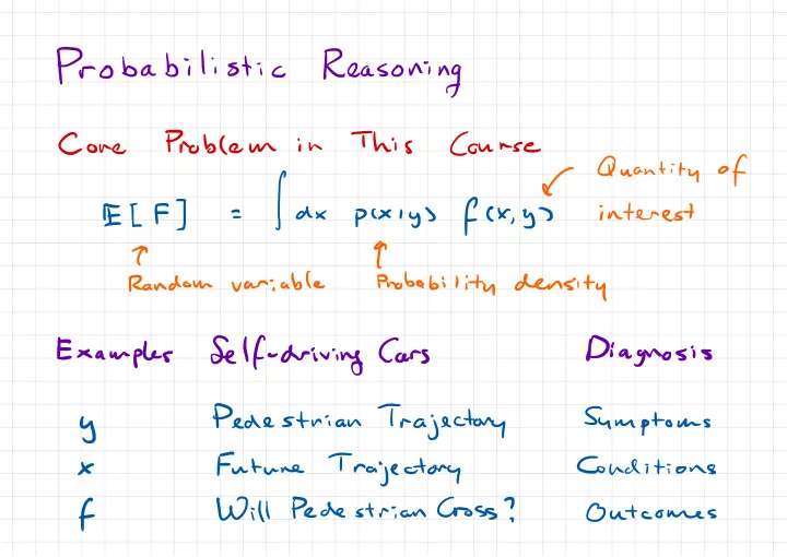
Cone
Problem
in
This
Course
f
Quantity
- f
fax
pcxiysfex.gs interest T t Random variable Probability density Examples Self- driving