
SLIDE 1
(fast) Randomized SVD
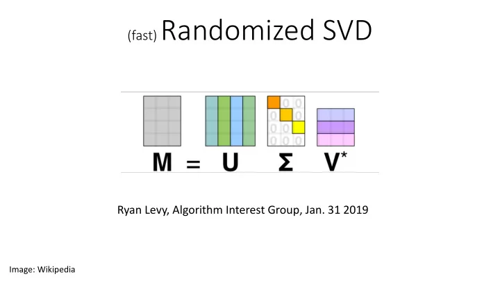
Ryan Levy, Algorithm Interest Group, Jan. 31 2019
Image: Wikipedia
(fast) Randomized SVD Ryan Levy, Algorithm Interest Group, Jan. 31 - - PowerPoint PPT Presentation
(fast) Randomized SVD Ryan Levy, Algorithm Interest Group, Jan. 31 2019 Image: Wikipedia Roadmap Review SVD Its awesome - why you should love it Singular values are almost math magic Bottleneck Scenarios the need for
Image: Wikipedia
That trick you learned in math class!
Singular Values Any Matrix
50% - 298 75% - 149 90% - 60 95% - 30
Key: [% Σ=0] – [# remaining]
Image: Wikipedia, doi:10.1038/nature15750
Large matrices take huge computational cost Sometimes have hundreds of large matrices to SVD (e.g. facebook)
Source: Facebook research
Passes through matrix
~complicated~
normalizing after each step Pro:
Cons:
components
convergence
✓ 0 M M † ◆ ✓U V ◆ = Σii ✓U V ◆
<latexit sha1_base64="(nul)">(nul)</latexit><latexit sha1_base64="(nul)">(nul)</latexit><latexit sha1_base64="(nul)">(nul)</latexit><latexit sha1_base64="(nul)">(nul)</latexit> Goal: obtain SVD for k singular values of a m x n matrix M, assuming m > n
c. Orthogonal matrix Q is m x k
Source: Halko, Martinsson and Tropp (2009)
B = uΣV †
<latexit sha1_base64="(nul)">(nul)</latexit><latexit sha1_base64="(nul)">(nul)</latexit><latexit sha1_base64="(nul)">(nul)</latexit><latexit sha1_base64="(nul)">(nul)</latexit>Random values are hopefully superposition of correct basis vectors “Randomized Range Finder”
Actual k=100 rSVD k=100 Thanks to smortezavi’s example code
Actual k=10 rSVD k=10 Thanks to smortezavi’s example code
Rounding error problem Instead do QR every step, alternate M, Mt
Actual k=100 rSVD k=100, q=1
Actual k=10 rSVD k=10, q=0 rSVD k=10, q=1 rSVD k=10, q=5 Timing (s): SVD: 0.613 rSVD q=0: 0.0096 rSVD q=1: 0.022
Actual k=10 rSVD k=10, q=0 rSVD k=10, q=20 Unstable rSVD k=10, q=20