Fairness and Optimal Stochastic Control for Heterogeneous Networks - - PowerPoint PPT Presentation

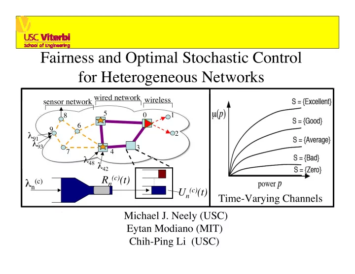
Fairness and Optimal Stochastic Control for Heterogeneous Networks

Time-Varying Channels

1 2 3 4 5 6 7 8 9

λ93 λ91 λ48 λ42

Un

(c)(t)

Rn

(c)(t)

λn

(c)

sensor network wired network wireless

Michael J. Neely (USC) Eytan Modiano (MIT) Chih-Ping Li (USC)

1 2 3 4 5 6 7 8 9

λ93 λ91 λ48 λ42

Un

(c)(t)

Rn

(c)(t)

λn

(c)

sensor network wired network wireless

A heterogeneous network with N nodes and L links: ΓS = ΓΑ

SA

ΓΒ ΓC

SC

= channel dependent set

• f transmission rate matrices

ΓS µ(t) ΓS(t) Choose t 0 1 2 3 … Slotted time t = 0, 1, 2, … Traffic (Aij(t)) and channel states S(t) i.i.d. over timeslots…

1 2 3 4 5 6 7 8 9

λ93 λ91 λ48 λ42

Un

(c)(t)

Rn

(c)(t)

λn

(c)

sensor network wired network wireless

A heterogeneous network with N nodes and L links:

Input rate matrix: (λij) (where E[Aij(t)] = λij) Channel state vector: S(t) = (S1(t), S2(t), …, SL(t))

ΓS = ΓΑ

SA

ΓΒ ΓC

SC

= channel dependent set

• f transmission rate vectors

ΓS

Transmission rate vector: µ(t) = (µ1(t), µ2(t), …, µL(t)) Resource allocation: choose µ(t) ΓS(t)

µ(t) ΓS(t) Choose

Goal: Develop joint flow control, routing, resource allocation

1 2 3 4 5 6 7 8 9

λ93 λ91 λ48λ42 Un

(c)(t)

Rn

(c)(t)

λn

(c)

sensor network wired network wireless

Λ = Capacity region (considering all routing, resource alloc. policies) gnc(rnc) = concave utility functions

util r

λ1 λ2

Some precedents: Static optimization: (Lagrange multipliers and convex duality) Kelly, Maulloo, Tan, Oper Res. 1998 [pricing for net. optimization] Xiao, Johansson, Boyd, Allerton 2001 [network resource opt.] Julian, Chian, O’Neill, Boyd, Infocom 2002 [static wireless opt] Lee, Mazumdar, Shroff, Infocom 2002 [static wireless downlink] Marbach, Infocom 2002 [pricing, fairness static nets] Krishnamachari, Ordonez, VTC 2003 [static sensor nets] Low, TON 2003 [internet congestion control] Dynamic control:

• D. Tse, 97, 99 [“proportional fair” algorithm: max Ui/ri]

Kushner, Whiting, Allerton 2002 [“prop. fair” alg. analysis]

• S. Borst, Infocom 2003 [downlink fairness for infinite # users]

Li, Goldsmith, IT 2001 [broadcast downlink] Tsibonis, Georgiadis, Tassiulas, Infocom 2003 [max thruput outside

• f capacity region]

Stochastic Stability via Lyapunov Drift: Tassiulas, Ephremides, AC 1992, IT 1993 [MWM, Diff. backlog] Andrews et. al., Comm. Mag, 2003 [server selection] Neely, Modiano, Rohrs, TON 2003, JSAC 2005 [satellite, wireless] McKeown, Anantharam, Walrand, Infocom 1996 [NxN switch] Leonardi et. Al., Infocom 2001 [NxN switch]

Example: Server alloc., 2 queue downlink, ON/OFF channels Pr[ON] = p1 Pr[ON] = p2 λ1 λ2

0.6

0.5

λ2 λ1

Capacity region Λ: MWM algorithm (choose ON queue with largest backlog) Stabilizes whenever rates are strictly interior to Λ [Tassiulas, Ephremides IT 1993]

Comparison of previous algorithms: (1) MWM (max Uiµi) (2) Borst Alg. [Borst Infocom 2003] (max µi/µi) (3) Tse Alg. [Tse 97, 99, Kush 2002] (max µi/ri)

1 2 3 4 5 6 7 8 9

λ93 λ91 λ48λ42 Un

(c)(t)

Rn

(c)(t)

λn

(c)

sensor network wired network wireless

Approach: Put all data in a reservoir before sending into

• network. Reservoir valve determines Rn(c)(t) (amount

delivered to network from reservoir (n,c) at slot t). Optimize dynamic decisions over all possible valve control policies, network resource allocations, routing to provide optimal fairness.

1 2 3 4 5 6 7 8 9

λ93 λ91 λ48λ42 Un

(c)(t)

Rn

(c)(t)

λn

(c)

sensor network wired network wireless

Part 1: Optimization with infinite demand Assume all active sessions infinitely backlogged (general case of arbitrary traffic treated in part 2).

λ2 λ1

Cross Layer Control Algorithm (CLC1): (1) Flow Control: At node n, observe queue backlogs Un

(c)(t)

for all active sessions c. Rest of Network

Un(c)(t)

Rn

(c2)(t)

λn

(c2)

Rn

(c1)(t)

λn

(c1)

(where V is a parameter that affects network delay)

(2) Routing and Scheduling: (similar to the original Tassiulas differential backlog routing policy [1992]) (

link l

cl*(t) = (3) Resource Allocation: Observe channel states S(t). Allocate resources to yield rates µ(t) such that:

l

Wl

*(t)µl(t)

Maximize: Such that: µ(t) ΓS(t)

Theorem: If channel states are i.i.d., then for any V>0 and any rate vector λ (inside or outside of Λ),

• Avg. delay:

Fairness: (where ) λ1

• ptimal point r *

µsym µsym

Special cases: (for simplicity, assume only 1 active session per node)

• 1. Maximum throughput and the threshold rule

Linear utilities: gnc(r) = αnc r

Un

(c)(t)

Rn

(c)(t)

λn

(c)

(threshold structure similar to Tsibonis [Infocom 2003] for a downlink with service envelopes)

(2) Proportional Fairness and the 1/U rule

logarithmic utilities: gnc(r) = log(1 + rnc)

Un

(c)(t)

Rn

(c)(t)

λn

(c)

Mechanism Design and Network Pricing:

Maximize: gnc(r) - PRICEnc(t)r

0 r Rmax

Such that :

greedy users…each naturally solves the following:

This is exactly the same algorithm if we use the following dynamic pricing strategy:

PRICEnc(t) = Unc(t)/V

g(r *)

C + VNGmax

• VE[g(r (t))|U(t)] - Vg(r *)

Theorem: (Lyapunov drift with Utility Maximization)

n

L(U(t)) = Un2(t) Δ(t) = E[L(U(t+1) - L(U(t)) | U(t)] Δ(t) C - ε

n Un(t)

Analytical technique: Lyapunov Drift Lyapunov function: Lyapunov drift:

If for all t: Then: (a)

n E[Un]

(stability and bounded delay) (b) g(rachieve ) + C/V (resulting utility) ε

Part 2: Scheduling with arbitrary input rates

λ1 λ2 Novel technique of creating flow state variables Znc(t)

Un

(c)(t)

Rn

(c)(t)

λn

(c)

Ync(t) = Rmax - Rnc(t) Znc(t) = max[Znc(t) - gnc(t), 0] + Ync(t) (Reservoir buffer size arbitrary, possibly zero)

the Znc(t+1) iteration of the previous slide. Cross Layer Control Alg. 2 (CLC2)

Simulation Results for CLC2: Pr[ON] = p1 Pr[ON] = p2 λ1 λ2 (i) 2 queue downlink a)g1(r)=g2(r)= log(1+r) b)g1(r)=log(1+r) g2(r)=1.28log(1+r) (priority service)

(ii) 3 x 3 packet switch under the crossbar constraint: .6 .1 .3 .2 0 .4 .5 proportionally fair

(iii) Multi-hop Heterogeneous Network

1 2 3 4 5 6 7 8 9

λ93 λ91 λ48 λ42

Un

(c)(t)

Rn

(c)(t)

λn

(c)

sensor network wired network wireless

λ91 = λ93 = λ48 = λ42 = 0.7 packets/slot (not supportable) Use CLC2, V=1000 ------> Utot =858.9 packets r91 = 0.1658, r93=0.1662, r48=0.1678, r42=0.5000 The optimally fair point of this example can be solved in closed form: r91* = r93* = r48* = 1/6 = 0.1667 , r42 = 0.5 Concluding Slide:

http://www-rcf.usc.edu/~mjneely/ The end