
SLIDE 1
Randomvariables
July 22g2020
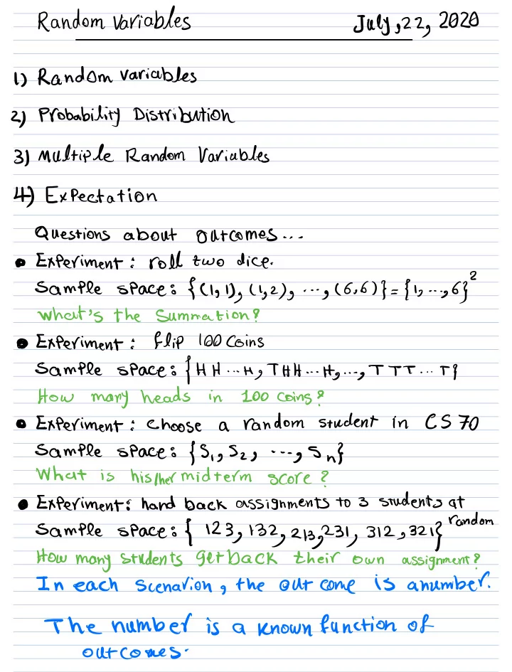
1 Random variables
2 Probability Distribution
3 Multiple Random Variables
4
Expectation
Questions
about
- utcomes
Experiment
roll
two dice
Sample space
ClgDsg Ig2 g
g 6.6
fly
63
What's the
summation
Experiment
flip
100Coins
Sample space fH H
HgTHA
Hg
g T TT
19 How many heads
in 100 Coins
Experiment
choose
a random student
in
CS 70 Sample space
f S g Szg
g S n
What
is
his her midterm
score
Experiment
E hand back assignments to 3 students at
random
Sample
space
1.23g132g213,231g 3123321
Howmany students get back
their
- wn
assignment
In
each
scenarion g the
- utcome
is
anumber
The
number is
a
known function of Outcomes