F ACTOR graph is a popular graphical model to represent where the - PDF document

FIRST YEAR REPORT 1 Generalization of Factor Graphs and Belief Propagation for Quantum Information Science Michael X. CAO Abstract —Factor graph is a useful tool to represent probability p u A u B q B b B b A systems. In this article, we propose a new factor graph model in representing quantum systems. Belief propagation algorithm is also generalized to this new model, and is justified via the method of loop calculus. 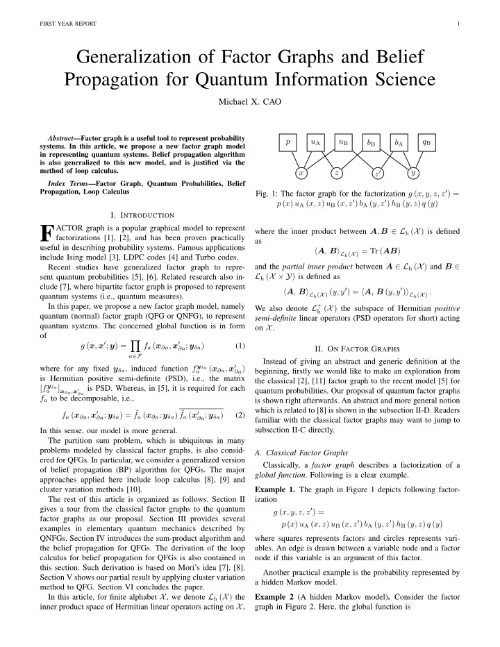y x z z ′ Index Terms —Factor Graph, Quantum Probabilities, Belief Propagation, Loop Calculus Fig. 1: The factor graph for the factorization g ( x, y, z, z ′ ) = p ( x ) u A ( x, z ) u B ( x, z ′ ) b A ( y, z ′ ) h B ( y, z ) q ( y ) I. I NTRODUCTION F ACTOR graph is a popular graphical model to represent where the inner product between A , B ∈ L h ( X ) is defined factorizations [1], [2], and has been proven practically as useful in describing probability systems. Famous applications � A , B � L h ( X ) = Tr ( AB ) include Ising model [3], LDPC codes [4] and Turbo codes. and the partial inner product between A ∈ L h ( X ) and B ∈ Recent studies have generalized factor graph to repre- L h ( X × Y ) is defined as sent quantum probabilities [5], [6]. Related research also in- clude [7], where bipartite factor graph is proposed to represent � A , B � L h ( X ) ( y, y ′ ) = � A , B ( y, y ′ ) � L h ( X ) . quantum systems (i.e., quantum measures). In this paper, we propose a new factor graph model, namely We also denote L + h ( X ) the subspace of Hermitian positive quantum (normal) factor graph (QFG or QNFG), to represent semi-definite linear operators (PSD operators for short) acting quantum systems. The concerned global function is in form on X . of g ( x , x ′ ; y ) = � f a ( x ∂a , x ′ ∂a ; y δa ) (1) II. O N F ACTOR G RAPHS a ∈F Instead of giving an abstract and generic definition at the ( x ∂a , x ′ where for any fixed y δa , induced function f y δa ∂a ) beginning, firstly we would like to make an exploration from a is Hermitian positive semi-definite (PSD), i.e., the matrix the classical [2], [11] factor graph to the recent model [5] for [ f y δa ] x ∂a , x ′ ∂a is PSD. Whereas, in [5], it is required for each quantum probabilities. Our proposal of quantum factor graphs a f a to be decomposable, i.e., is shown right afterwards. An abstract and more general notion which is related to [8] is shown in the subsection II-D. Readers f a ( x ∂a , x ′ ∂a ; y δa ) = ˜ f a ( x ∂a ; y δa ) ˜ f a ( x ′ ∂a ; y δa ) (2) familiar with the classical factor graphs may want to jump to subsection II-C directly. In this sense, our model is more general. The partition sum problem, which is ubiquitous in many problems modeled by classical factor graphs, is also consid- A. Classical Factor Graphs ered for QFGs. In particular, we consider a generalized version Classically, a factor graph describes a factorization of a of belief propagation (BP) algorithm for QFGs. The major global function . Following is a clear example. approaches applied here include loop calculus [8], [9] and cluster variation methods [10]. Example 1. The graph in Figure 1 depicts following factor- The rest of this article is organized as follows. Section II ization gives a tour from the classical factor graphs to the quantum g ( x, y, z, z ′ ) = factor graphs as our proposal. Section III provides several p ( x ) u A ( x, z ) u B ( x, z ′ ) b A ( y, z ′ ) h B ( y, z ) q ( y ) examples in elementary quantum mechanics described by QNFGs. Section IV introduces the sum-product algorithm and where squares represents factors and circles represents vari- the belief propagation for QFGs. The derivation of the loop ables. An edge is drawn between a variable node and a factor calculus for belief propagation for QFGs is also contained in node if this variable is an argument of this factor. this section. Such derivation is based on Mori’s idea [7], [8]. Another practical example is the probability represented by Section V shows our partial result by applying cluster variation a hidden Markov model. method to QFG. Section VI concludes the paper. In this article, for finite alphabet X , we denote L h ( X ) the Example 2 (A hidden Markov model) . Consider the factor inner product space of Hermitian linear operators acting on X , graph in Figure 2. Here, the global function is

FIRST YEAR REPORT 2 x 0 x 1 x 2 x 3 X Y U B H = = y 1 y 2 y 3 p ( x ) U H B p Y | X ( y | x ) Fig. 2: Normal factor graph for a hidden Markov model of length 3 Fig. 4: Factor graph for an elementary quantum system z u A b B B. Factor Graphs for Quantum Probabilities y x p = = q Factor graphs can be used to represent quantum probabilities if more general factors are allowed [5], [6]. Following is an u B b A z ′ example as a modification of Example 3. Example 4. Consider the factor graph in Figure 4. Here, some of the factors are given in matrix form. The dots at the end of Fig. 3: Normal factor graph for the first example each edges are used to specify which variable is performing as the first index of the matrix. In this case, the global function x ′ ) g ( x, y, ˜ x, ˜ 3 � p ( y 1 , . . . , y 3 , x 0 , . . . , x 3 ) = p 0 ( x 0 ) p k ( y k , x k | x k − 1 ) . x, x ) U H ( x, ˜ x ′ ) B H ( y, ˜ x ′ , y ) � p ( x ) U (˜ x ) B (˜ k =1 x ′ , y ) U (˜ x ′ , x ) B (˜ = p ( x ) U (˜ x, x ) B (˜ x, y ) (3) In this case, x 0 , x 1 , . . . are the hidden variables. Note that in where U and B are both complex unitary matrices. above factor graph, the nodes for the variables are omitted, Though we have complex-valued functions as factors in this since each variable is only connected to at most two factors. cases, the marginal functions can still be real-nonnegative, due A factor graph with variables represented by edges directly to the symmetric structure. For example, by closing the box is called a normal factor graph [1], [11], [12]. The notion in Figure 4, we have following exterior function of normal factor graph is not only generic (as shown in next � x ′ , y ) U (˜ p Y | X ( y | x ) = U (˜ x, x ) B (˜ x ′ , x ) B (˜ x, y ) example), but also provide extra benefits by introducing the x ′ concept of “opening/closing the box” [1], [5], [6]. x, ˜ ˜ � � = U (˜ x, x ) B (˜ x, y ) · U (˜ x ′ , x ) B (˜ x ′ , y ) Example 3. This example shows the conversion of a standard ˜ x x ′ ˜ factor graph into a normal factor graph by adding extra “equal” 2 � � factor nodes. Figure 3 depicts the corresponding normal factor � � � = U (˜ x, x ) B (˜ x, y ) � � graph for Example 1, where two “equal” factor nodes are � � � � x ˜ added to make duplications of variables x and y , respectively. which exactly describes the conditional probability of variable Now, consider the dashed box in Figure 2. We define the Y given X in a quantum system with one-time unitary exterior function of such a box as the product of all factors evolution and a single projective measurement [13]. inside the box summing over all internal variables. For this Consider the factor graphs constructed in a symmetric example, we have the exterior function as manner where complex functions always appear in conjugate p Y 1 ,Y 2 ,Y 3 | X 0 ( y 1 , y 2 , y 3 | x 0 ) = pairs, as in Example 4. In this case, any factorization with � constrain in equation (2) is representable, in particular, a p ( x 0 ) p ( y 1 , x 1 | x 0 ) p ( y 2 , x 2 | x 1 ) p ( y 3 , x 3 | x 2 ) . variety of a quantum systems are included [5], [6]. x 1 ,x 2 ,x 3 Note that the exterior function is always a functions of C. Quantum Factor Graphs (QFGs) the variables crossing the box boundary. By replacing the 1) Redraw of example 4: box with a factor corresponding to its exterior function, the Example 5. Consider the factor graph in Figure 5 as a redraw resultant factor graph yields a new factorization with less of Figure 4, where each factor here is given by a matrix with variables. In this case, the marginals with respect to (w.r.t.) the combination of the upper-edge variables as the first index. the remaining variables will keep unchanged. Such operation The dot notation in this case is used in a different manner: is often refereed to as “ closing-the-box ”, whereas its reverse It is applied to clarify the order between upper (lower)-edge is called “ opening-the-box ” [1], [5], [6]. variables in nesting-up of the first (second) index. In this case, The operation of “closing-the-box” is closely related to the factors in red and blue can be respectively written as the idea of sum-product algorithm [2] where a sequence of “closing-the-box” operation are taken in order. However, as ˆ x ′ , x ′ ) � � � U (˜ (˜ x, x ) , (˜ x, x ) · U (˜ x ′ , x ′ ) U presented in next subsection, such operation is not limited to ˆ x ′ , ˜ y ′ ) x ′ , ˜ y ′ ) . � � � B (˜ (˜ x, ˜ y ) , (˜ x, ˜ y ) · B (˜ B traditional probability models.