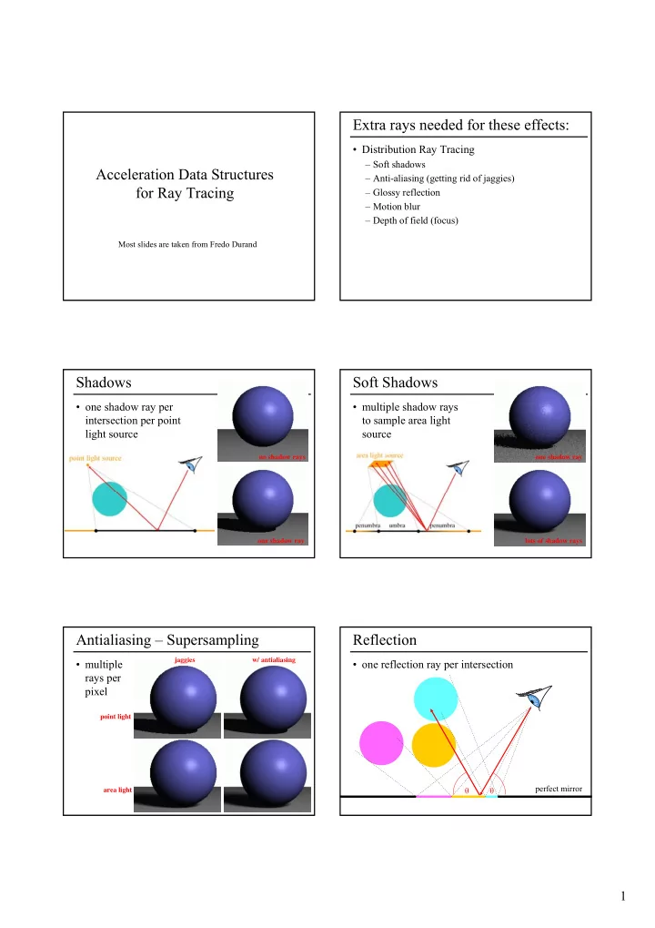
Extra rays needed for these effects: Distribution Ray Tracing - PDF document

Extra rays needed for these effects: • Distribution Ray Tracing – Soft shadows Acceleration Data Structures – Anti-aliasing (getting rid of jaggies) for Ray Tracing – Glossy reflection – Motion blur – Depth of field (focus) Most slides are taken from Fredo Durand Shadows Soft Shadows • one shadow ray per • multiple shadow rays intersection per point to sample area light light source source no shadow rays one shadow ray one shadow ray lots of shadow rays Antialiasing – Supersampling Reflection jaggies w/ antialiasing • multiple • one reflection ray per intersection rays per pixel point light perfect mirror θ θ area light 1

Glossy Reflection Motion Blur • multiple reflection • Sample objects rays temporally Justin Legakis polished surface θ θ Rob Cook Algorithm Analysis The Ray Tree • Ray casting cost ≤ height * width * T 3 • Lots of primitives num primitives * Eye R 2 intersection cost * • Recursive N 2 T 1 R 3 num shadow rays * R 1 N 3 • Distributed Ray supersampling * L 1 Tracing Effects num glossy rays * L 2 N 1 L 3 L 1 num temporal samples * R 1 T 1 – Soft shadows max recursion depth * – Anti-aliasing . . . L 2 L 3 N i surface normal – Glossy reflection Eye R 2 R 3 T 3 R i reflected ray – Motion blur can we reduce this? L i shadow ray – Depth of field T i transmitted (refracted) ray Questions? Accelerating Ray Tracing • Four main groups of acceleration techniques: – Reducing the average cost of intersecting a ray with a scene: • Faster intersection calculations • Fewer intersection calculations – Reducing the total number of rays that are traced • Adaptive recursion depth control – Discrete Ray Tracing • proximity clouds – Using generalized rays – Parallelization, specialized hardware 2

Acceleration of Ray Casting Bounding Volumes • Goal: Reduce the • Idea: associate with each object a simple bounding volume. If a ray misses the bounding volume, it also number of misses the object contained therein. ray/primitive • Common bounding volumes: intersections – spheres – bounding boxes – bounding slabs • Effective for additional applications: – Clipping acceleration – Collision detection • Note: bounding volumes offer no asymptotic improvement! Conservative Bounding Region Conservative Bounding Regions • First check for an • tight → avoid bounding sphere intersection with a false positives conservative • fast to intersect bounding region • Early reject non-aligned bounding box axis-aligned bounding box arbitrary convex region (bounding half-spaces) Bounding Volumes Bounding Boxes can overlap 3

Intersection with Axis-Aligned Box Bounding Volume Hierarchy • Introduced by James Clark (SGI, Netscape) in From Lecture 3, • For all 3 axes, Ray Casting II 1976 for efficient view-frustum culling. calculate the intersection distances t 1 and t 2 • t near = max ( t 1x , t 1y , t 1z ) t 2x t far = min ( t 2x , t 2y , t 2z ) t far y=Y2 Procedure IntersectBVH(ray, node) • If t near > t far , begin t 2y if IsLeaf(node) then box is missed Intersect(ray, node.object) t nea r t 1x • If t far < t min , else if IntersectBV(ray,node.boundingVolume) box is behind then foreach child of node do y=Y1 • If box survived tests, IntersectBVH(ray, child) t 1y endfor report intersection at t near x=X2 x=X1 endif end Bounding Volume Hierarchy Bounding Volume Hierarchy • Find bounding box of objects • Find bounding box of objects • Split objects into two groups • Split objects into two groups • Recurse • Recurse Bounding Volume Hierarchy Bounding Volume Hierarchy • Find bounding box of objects • Find bounding box of objects • Split objects into two groups • Split objects into two groups • Recurse • Recurse 4

Bounding Volume Hierarchy Where to split objects? • Find bounding box of objects • At midpoint OR • Sort, and put half of the objects on each side OR • Split objects into two groups • Use modeling hierarchy • Recurse Intersection with BVH Intersection with BVH • Check subvolume with closer intersection first • Don't return intersection immediately if the other subvolume may have a closer intersection Questions? Spatial Subdivision • Uniform spatial subdivision: – The space containing the scene is subdivided into a uniform grid of cubes “voxels”. – Each voxel stores a list of all objects at least partially contained in it.in – Given a ray, voxels are traversed using a 3D variant of the 2D line drawing algorithms. – At each voxel the ray is tested for intersection with the primitives stored therein – Once an intersection has been found, there is no need to continue to other voxels. 5

Regular Grid Create grid • Find bounding Cell ( i, j ) box of scene • Choose grid spacing • grid x need not = grid y grid y grid x Insert primitives into grid For each cell along a ray • Primitives • Does the cell that overlap contain an multiple intersection? cells? • Yes: return • Insert into closest multiple intersection cells (use • No: continue pointers) Preventing repeated computation Don't return distant intersections • Perform the • If intersection computation t is not within once, "mark" the cell range, the object continue (there may be • Don't something re-intersect closer) marked objects 6

Where do we start? Is there a pattern to cell crossings? • Intersect ray • Yes, the Cell ( i, j ) with scene horizontal bounding box and vertical crossings • Ray origin dt v = grid y / dir y have regular may be inside spacing the scene bounding box t next_h t next_v t next_v t min grid y t next_h dt h = grid x / dir x t min ( dir x , dir y ) grid x What's the next cell? What's the next cell? • 3DDDA – Three if t next_v < t next_h Cell ( i+ 1 , j ) Dimensional Digital i += sign x Cell ( i, j ) Difference Analyzer t min = t next_v t next_v += dt v else • We'll see this t next_h again later, for j += sign y t next_v line rasterization t min = t next_h t min t next_h += dt h dt h dt v ( dir x , dir y ) if (dir x > 0) sign x = 1 else sign x = -1 if (dir y > 0) sign y = 1 else sign y = -1 Pseudo-code Regular Grid Discussion • Advantages? create grid insert primitives into grid – easy to construct for each ray r – easy to traverse find initial cell c(i,j), t min , t next_v & t next_h compute dt v , dt h , sign x and sign y • Disadvantages? while c != NULL for each primitive p in c – may be only sparsely filled intersect r with p – geometry may still be clumped if intersection in range found return c = find next cell 7

Questions? Adaptive Grids • Subdivide until each cell contains no more than n elements, or maximum depth d is reached Nested Grids Octree/(Quadtree) Primitives in an Adaptive Grid Top down traversal • Can live at intermediate levels, or be pushed to lowest level of grid Split ray into sub-segments and traverse each segment recursively. Octree/(Quadtree) Bottom Up traversal Kd-trees vs. Quad-tree Step from cell to cell. Intersect current cell and add an epsilon into the next cell. Then search for the cell in the tree. A naïve search starts from the root. Otherwise, try an intelligent guess… 8

Kd-trees vs. BSP-tree Adaptive Spatial Subdivision • Disadvantages of uniform subdivision: – requires a lot of space – traversal of empty regions of space can be slow – not suitable for “teapot in a stadium” scenes • Solution: use a hierarchical adaptive spatial subdivision data structure – octrees – BSP-trees • Given a ray, perform a depth-first traversal of the tree. Again, can stop once an intersection has been found. Bounding Volume Hierarchy Discussion Uniform vs. Adaptive Subdivision • Advantages – easy to construct – easy to traverse – binary • Disadvantages – may be difficult to choose a good split for a node – poor split may result in minimal spatial pruning Macro-regions Proximity Clouds 9

Parallel/Distributed RT • Two main approaches: – Each processor is in charge of tracing a subset of the rays. Requires a shared memory architecture, replication of the scene database, or transmission of objects between processors on demand. – Each processor is in charge of a subset of the scene (either in terms of space, or in terms of objects). Requires processors to transmit rays among themselves. Directional Techniques Directional Techniques • Ray classification (Arvo and Kirk 87): – Rays in 3D have 5 degrees of freedom: (x,y,z, θ,φ ) • Light buffer: accelerates shadow rays. – Rays coherence: rays belonging to the same small 5D neighborhood are likely to intersect the same set of objects. – Discretize the space of directions around each – Partition the 5D space of rays into a collection of 5D light source using the direction cube hypercubes, each containing a list of objects. – In each cell of the cube store a sorted list of – Given a ray, find the smallest containing 5D hypercube, and objects visible from the light source through that test the ray against the objects on the list. cell – For efficiency, the hypercubes are arranged in a hierarchy: a 5D analog of the 3D octree. This data structure is constructed – Given a shadow ray locate the appropriate cell of in a lazy fashion. the direction cube and test the ray with the objects on its list 10