Example: PCA of a matrix of fatty acids in margarines 1.0 C12 0.8 - - PowerPoint PPT Presentation

R algorithms for the calculation of markers to be used in the construction of predictive and interpolative biplot axes in routine multivariate analyses

• M. Rui Alves 1,2 and M. Beatriz Oliveira 2

(1) Escola Superior de Tecnologia e Gestão, IPVC, Viana do Castelo, Portugal

(2) REQUIMTE, Faculdade de Farmácia, Universidade do Porto, Porto, Portugal

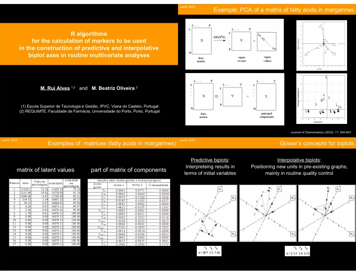
Example: PCA of a matrix of fatty acids in margarines

Principal component 1

Principal component 2

A1 A2 A3 A4 A5 B1 B2 B3 B4 B5 C1 C2C3 C4 C5 D1 D2 D3 D4 D5 E1 E2 E3 E4 E5 F1 F3 F4 F5 G1 G2 G3 G4 G5 H1 H2 H3 H4 H5

• 10

10 20 30 40

• 40
• 30
• 20
• 10

10 20 30 Latent vector 1

Latent vector 2

• 1.0
• 0.8
• 0.6
• 0.4
• 0.2

0.0 0.2 0.4 0.6 0.8 1.0

• 1.0
• 0.8
• 0.6
• 0.4
• 0.2

0.0 0.2 0.4 0.6 0.8 1.0 C18:2cc (-0.75 ; -0.40) Ttr (0.19 ; -0.28) C18:1c (0.42 ; -0.43) C16 (0.46 ; -0.01) C12 (-0.08 ; 0.72) C14 (-0.01 ; 0.19) C18 (-0.04 ; -0.10)

Journal of Chemometrics (2003), 17, 594-602 useR! 2006

Examples of matrices (fatty acids in margarines) matrix of latent values part of matrix of components

useR! 2006

Gower’s concepts for biplots

Predictive biplots: Interpreteing results in terms of initial variables Interpolative biplots: Positioning new units in pre-existing graphs, mainly in routine quality control

useR! 2006

PCA biplots: fatty acids in margarines

Predictive biplots Interpreting results Interpolative biplots Positioning new units

Journal of Chemometrics (2001), 15, 71-84 Journal of Chemometrics (2003), 17, 594-602 useR! 2006

Problems on computation

• Gower e Hand, in their book Biplots, say:

“(...) The main computational problems [of biplots] are in integrating different bits of available software and in finding good portable graphic facilities.

• To work with bipots we used:

– Genstat 5.3.1 package to develop the algorithms and carry out the analyses – Statistica for Windows to draw all the graphs based on the converted ASCII outputs produced by Genstat

• We started to work with R in an attempt to provide a final, complete

and more covenient solution

useR! 2006

Projection of markers

Projection of Markers

[ μ p− 1

x p s p

− 1][e p t V ρ − 1 t

][e p

t V ρ − 1 t

V ρ

− 1e p] − 1

[ μ p− 1

x p s p

− 1][e p t V ρ] useR! 2006

Building biplots (PCA of fatty acids in sunflower oils)

Componente principal 1

Componente principal 2

1 2 3 4 5 6 7 8 9 10 11 12 13 14 15 16 17 18 19 20 21 22 23 24 25 26 27 28 29 30 31 32 33 34 35 36 37 38 39 40 41 42 43 44 45 46 47 48 49 50 51 52 53 54

• 7
• 6
• 5
• 4
• 3
• 2
• 1

1 2 3 4 5 6 7

• 7
• 6
• 5
• 4
• 3
• 2
• 1

1 2 3 4 5 6 7 Componente principal 1

Componente principal 2

1 2 3 4 5 6 7 8 9 10 11 12 13 14 15 16 17 18 19 20 21 22 23 24 25 26 27 28 29 30 31 32 33 34 35 36 37 38 39 4041 42 43 44 45 46 47 48 49 50 51 52 53 54

56 58 60 62 64

• 7
• 6
• 5
• 4
• 3
• 2
• 1

1 2 3 4 5 6 7

• 7
• 6
• 5
• 4
• 3
• 2
• 1

1 2 3 4 5 6 7 C 18:2cc componente 1

componente 2

• 10
• 8
• 6
• 4
• 2

2 4 6 8 10

• 10
• 8
• 6
• 4
• 2

2 4 6 8 10 variáveis muito longas 5.0 5.5 6.0 6.5 7.0 0.05 0.10 0.15 0.20 24.5 26.5 28.5 30.5 56 58 60 62 64 0.28 0.30 0.32 0.34 0.36 C 16 C 16:1 C 18:1 C 18:2 C 20

useR! 2006

Strategies for the automation of the process

Two strategies were devised: The first, more obvious, is to create an object containing the markers, the axis, the scale values and variable’s name.

• Project the object.
• Live it in the graph if it fits well
• Delete it otherwise (too long or too short vectors)
• This procedure would require interactivity facilities

The second, more mathematical:

• Find a way for the evaluation of variables’ predictive powers
• Leave in the graph variables displaying high predictive power
• Delete them otherwise
• Draw the graphs (only with automatically selected variables)

useR! 2006

Algorithm for the selection based on predictive powers un  pred =read in the graph=0,5 un inicial =initial value=0,4 erro

u n=0,5− 0,4=0,1

erro

 x p=1

N ∑n=1

N

un pred− unincial s p Define a tolerance value if error

x p¿ tolerance⇒accept x p

if errorx p¿ tolerance⇒reject x p

useR! 2006

Pr ediction=X ⊗V 2dim ⊗V [k ,]

2 dimt

UnitsStdE=abs  X [ ,k ]− Pr ediction MeanStdE=N − 1×1t ⊗UnitSdtE

Evaluation of predictive power and decision

if MeanStdETolerance  project var iable else pr int ital deleted 

[ μ p− 1

x p s p

− 1][e p t V ρ − 1 t

][e p

t V ρ − 1 t

V ρ

− 1e p] − 1

useR! 2006

for (i in 1:(Q-1)) { for (j in (i+1):Q) { print("component"); print(i); print("component"); print(j) # latent variables for a pair of components only V2Dim[,1] <- RedV[,i] V2Dim[,2] <- RedV[,j] MStdE <- list() for (k in 1:P) { # evaluation of variable' s predictive power print("variavel") ; print(k) VarDir <- matrix(data=(V2Dim[k,]),nrow=1,ncol=2) Pred <- XStd %*% V2Dim %*% t(VarDir) UnitStdE <- abs(XStd[,k] - Pred) VarE <- (t(ColN1s) %*% UnitStdE)/N MStdE[[k]] <- VarE print(MStdE[[k]]) if (MStdE[[k]] < Tolerance) { Zeros <- matrix(0,c(P,1)) Zeros[k,] <- 1 Adj1 <- t(Zeros) %*% V2Dim %*% t(V2Dim) %*% Zeros Adj2 <- (ColM1s %*% (1/Adj1) %*% t(Col2_1s)) EPred <- Adj2 * (ScMat[[k]] %*% V2Dim) print(EPred) plot(EPred[,1],EPred[,2]) } else print("deleted") } } }

useR! 2006

[1] "component" [1] 1 [1] "component" [1] 2 [1] "variavel" [1] 1 [,1] [1,] 0.6583496 [1] "deleted" [1] "variavel" [1] 2 [,1] [1,] 0.5805472 [1] "deleted" [1] "variavel" [1] 3 [,1] [1,] 0.2413512 [,1] [,2] [1,] 2.6066496 4.1854190 [2,] 1.4223328 2.2837971 [3,] 0.2380160 0.3821751 [4,] -0.9463008 -1.5194468 [5,] -2.1306176 -3.4210688

Example of results provided by the algorithm

useR! 2006

What needs to be done and acknowledgments

• Reminding Gower and Hand: “(...) The main computational

problems [dos biplots] are in integrating different bits of available software and in finding good portable graphic facilities.

• The algorithms are done, although probably not in the best or more

efficient way, but they provide correct results

• Produce biplots by making the graphs of components and merging

the graphs of individual variables as objects

• Multivariate analyses can therefore be made fully automatic,

including the interpretation processes

• Paul Murrell and Robert Gittins provided valuable information on

graphs and strategies to finalize the work, but unfortunately we did not find the time necessary to do it

useR! 2006

Thank you

useR! 2006