Evolutionary game theory for biologists Population dynamics Manual - - PowerPoint PPT Presentation

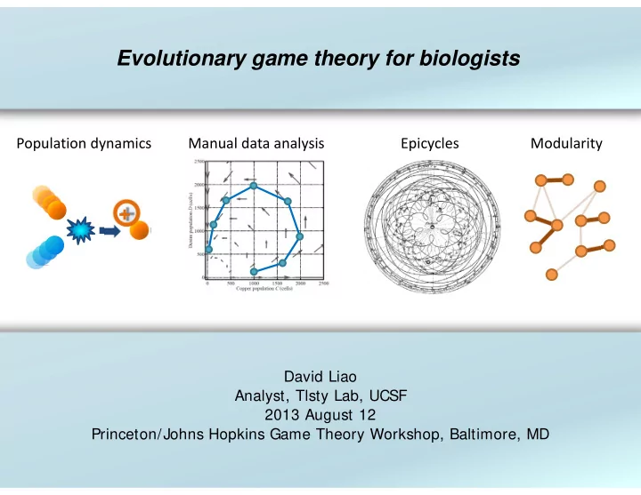
Epicycles Manual data analysis Population dynamics Modularity

+

David Liao Analyst, Tlsty Lab, UCSF 2013 August 12 Princeton/Johns Hopkins Game Theory Workshop, Baltimore, MD

Evolutionary game theory for biologists

Basic model with pairwise interactions

2

• Population dynamics

Note: Using labels C, D, T, R, P, and S does not, itself, logically imply that this model be a “prisoner’s dilemma”

Manual data analysis Epicycles Population dynamics Modularity

+ Evolutionary game theory for biologists

David Liao Analyst, Tlsty Lab, UCSF 2013 August 12 Princeton/Johns Hopkins Game Theory Workshop, Baltimore, MD

Back-of-the-envelope data analysis

4

Estimating rate coefficient from initial slope

5

(a) Estimate the parameters T, R, P, and S. Express your answers in units of day‐1.

• (if pC ~ 1)

1

• ∆

∆ Seeded 10,000 copper cells and only 100 denim cells 1 10,000 cells 5000 cells 2 days +5000 cells +2 days 1 4 day T = 0.5 day‐1; R = 0.25 day‐1; P = ‐0.25 day‐1; S = ‐0.5 day‐1

Using a model to fill in a phase plane

6

(b) Draw quivers on the provided sheet of graph paper to approximate how much the copper and denim subpopulations would change over the course of a day, starting from various initial subpopulation sizes.

• Start from C = D = 2000, find population change over a day?

∆ ∆ ∆ 0.25 day 0.5 0.5 day 0.5 2000 cells 1 day ∆ 250 cells ∆ ∆ ∆

• 0. 5 day

0.5 0.25 day 0.5 2000 cells 1 day ∆ 250 cells

T = 0.5 day‐1; R = 0.25 day‐1; P = ‐0.25 day‐1; S = ‐0.5 day‐1

Using a model to fill in a phase plane

7

(b) Draw quivers on the provided sheet of graph paper to approximate how much the copper and denim subpopulations would change over the course of a day, starting from various initial subpopulation sizes.

• From C = D = 2000,

T = 0.5 day‐1; R = 0.25 day‐1; P = ‐0.25 day‐1; S = ‐0.5 day‐1

∆ ∆ ∆ 250 cells ∆ ∆ ∆ 250 cells

Using a model to fill in a phase plane

8

(b) Draw quivers on the provided sheet of graph paper to approximate how much the copper and denim subpopulations would change over the course of a day, starting from various initial subpopulation sizes.

• From C = D = 2000,

T = 0.5 day‐1; R = 0.25 day‐1; P = ‐0.25 day‐1; S = ‐0.5 day‐1

∆ ∆ ∆ 250 cells ∆ ∆ ∆ 250 cells

Back-of-the-envelope data analysis

9

Validating model using phase path

10

(c) Represent the data from container III as a phase path in the phase plane you have just sketched. Is the trajectory consistent with the quiver field in direction and magnitude?

Back-of-the-envelope data analysis

11

Momentum is conserved A mixture of cell subpopulations proliferates with fitnesses linearly dependent on population composition Recently, ideas about complexity, self-organization, and emergence--when the whole is greater than the sum of its parts--have come into fashion as alternatives for metaphors

• f control. But such explanations offer only smoke and

mirrors, functioning merely to provide names for what we can't explain; they elicit for me the same dissatisfaction I feel when a physicist says that a particle's behavior is caused by the equivalence of two terms in an equation. . . . The hope that general principles will explain the regulation

• f all the diverse complex dynamical systems that we find in

nature can lead to ignoring anything that doesn't fit a pre-existing model. When we learn more about the specifics of such systems, we will see where analogies between them are useful and where they break down.

• -Deborah Gordon (2007)

Control without hierarchy. Nature 446: 143

Manual data analysis Epicycles Population dynamics Modularity

+ Evolutionary game theory for biologists

David Liao Analyst, Tlsty Lab, UCSF 2013 August 12 Princeton/Johns Hopkins Game Theory Workshop, Baltimore, MD

• ⋯

Mass action, Taylor series, and epicycles

13

• Population dynamics

Pairwise collisions 3‐way collisions ≥ 4‐way Power‐series for generic analytic function

Manual data analysis Epicycles Population dynamics Modularity

+ Evolutionary game theory for biologists

David Liao Analyst, Tlsty Lab, UCSF 2013 August 12 Princeton/Johns Hopkins Game Theory Workshop, Baltimore, MD

How complicated must our model be?

15

Intracellular 2 cell subpopulations 3 cell subpopulations . . . Patient

Mouse sketch file (and CC BY SA license information) at commons.wikimedia.org/wiki/File:Vectorized_lab_mouse_mg_3263_for_scientific_figures_and_presentations.svg

Modularity

16

Given risks and economics, should compartments be tightly connected or well isolated? Sophisticated computation Fault containment, revision Burn coal Power engine Turn propellers Keep water out How does time‐varying environment in which life evolves determine scale(s) at which and mechanisms by which a system is integrated and/or segregated?

Manual data analysis Epicycles Population dynamics Modularity

+ Evolutionary game theory for biologists

David Liao Analyst, Tlsty Lab, UCSF 2013 August 12 Princeton/Johns Hopkins Game Theory Workshop, Baltimore, MD

+

Questions

• Acknowledgments

NIH/NCI U54CA143803 (Austin) Thea Tlsty/Tlsty Lab Mechanisms Direct contact Indirect contact: Short‐lived soluble factor This validation of a mutation‐free model also validates model with mutation

• Compare results from 2‐, 3‐, 4‐subpopulation

experiments to infer modularity? Motifs vs. modules Kashtan & Alon 2005 Huang & Kauffman 2013 Why doesn’t

• rigin look like a

saddle?

+

Validation of mutation-free model consistent with social mutation

• In this example, S = ‐T
• Let T = k1 – k2
• Socially modulated mutation