[PDF] - A Nonparametric Bayesian Basket Trial Slide 4 Design Report PDF Document

SLIDE 1

Slide 1

A Nonparametric Bayesian Basket Trial Design

Peter M¨ uller, UT Austin www.math.utexas.edu/users/pmueller/oncostat.pdf

¡ ¡ ¡round ¡1 ¡ ¡ ¡ ¡ ¡round ¡3 ¡ Biomarker ¡1 ¡ Biomarker ¡1 ¡ Biomarker ¡1 ¡ Biomarker ¡1 ¡ Biomarker ¡2 ¡ Biomarker ¡2 ¡ Biomarker ¡2 ¡ Biomarker ¡2 ¡

S1 L1 S1 LL12 LS12 SS11 SL11 LL12

LSL121 LSS121

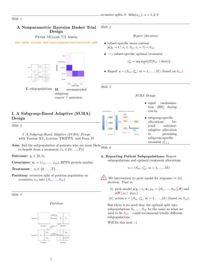
I. subpopulations

II. recommended subgroup cancer × mutation

I. A Subgroup-Based Adaptive (SUBA)

Design

Slide 2

I. A Subgroup-Based Adaptive (SUBA) Design

with Yanxun XU, Lorenzo TRIPPA, and Yuan JI Aim: find the subpopulation of patients who are most likely to benefit from a treatment (zi ∈ {0, . . . , T}) Outcome: yi ∈ {0, 1} Covariates: xi = (xi1, . . . , xip), RPPA protein marker. Treatment: zi ∈ {0, . . . , T}. Partition: recursive split of patition population on covariates xij into {S1, . . . , SM} Slide 3 Partition

¡ ¡ ¡round ¡1 ¡ ¡ ¡ ¡ ¡round ¡3 ¡ Biomarker ¡1 ¡ Biomarker ¡1 ¡ Biomarker ¡1 ¡ Biomarker ¡1 ¡ Biomarker ¡2 ¡ Biomarker ¡2 ¡ Biomarker ¡2 ¡ Biomarker ¡2 ¡

S1 L1 S1 LL12 LS12 SS11 SL11 LL12

LSL121 LSS121

recursive splits @ Mdn(xjs), s = 1, 2, 3 Slide 4 Report (decision)

subset-specific mean outome

p(yi = 1 | xi ∈ Sm, zi = t) = θmt

−

→ subset-specific optimal treatment z⋆

m = arg max t {E(θmt | data)}

Report a = (Sm, z⋆

m; m = 1, . . . , M) (based on θmt)

Slide 5 SUBA Design

equal

randomiza- tion (ER) during run-in;

subgroup-specific

allocations be- yond:

utcome-

adaptive allocation to promising subgroup-specific treament z⋆

n+1

Slide 6

4. Reporting Patient Subpopulations: Report

subpopulations and optimal treatment allocations a = (Sm, z⋆

m; m = 1, . . . , M)

! We intertwined (i) prob model for response ↔ (ii)

decision. That is,

(i) prob model p(yi | zi, xi, ρn = {S1, . . . , SM}, θ) and p(θ | ρn) · p(ρn) (ii) action a = (Sm, z⋆

m; m = 1, . . . , M) (based on θmt)

But there is no need that the optimal split into subpopulations S1, . . . , SM be the same as what we used to fit θmt – could recommend totally different subpopulations. Will fix this next :-) 1

SLIDE 2

II. IMPACT II: a basket trial for targeted

therapy

Slide 7

II. IMPACT II: a basket trial for targeted therapy

with Yanxun Xu, Don Berry and A. Tsimboridou Trial: study of targeted agents in metastatic cancers. Patients: metastatic cancer (thyroid, ovarian, melanoma, lung . . .) Treatments: therapy that targets particular molecular aberrations (TT) vs. standard of care (S) Population finding: yi = PFS; heterogeneous pat population – xi = different mutations; different cancers; baseline covs . . . Treatment might be effective for a subgroup across diseases Strategy (for pop. finding): similar to (I), but separate (i) prob model p(y | x, θ), vs. (ii) decision problem a ∈ A.

1 Decision problem

Slide 8

2. Decision Problem

Actions: Report a (i.e., one) subgroup of patients who might most benefit from TT: a : patients with xijk = x⋆

jk, k = 1, . . . , K

select (multiple) combination of mutations and cancer Prob model: (indexed by θ) Decision problem: separate inference (predicting PFS) vs. decision (report subpopulation).

no need for multiplicity control
arbitrary prob model
disentagle stat significance vs. clinical relevance
allow for variable # covs.

Slide 9 Utility: we favor a subpopulation with difference (relative to the overall population) in log hazards ratio (HR), large size and parsimonious description with few covariates, u(a, θ) = (HR(a, θ) − β) · n(a)α (|I| + 1)γ with n(a) = size of the subpopulation, and θ indexes the sampling model, Bayes rule: Report a⋆ = arg maxa

u(a, θ) dp(θ | data)
U(a)

, maximizing expected utility U(a). Alternative utility: Foster, Taylor & Ruberg (2011, StatMed) use Q(A) = enhanced treatment effect − average trt effect and sensitivity and specificity to evaluate a reported subpopulation A. Model: Decicsion problem and solution remain meaningful for any model, e.g. a nonparametric Bayes model (“always right”)

2 Simulation

Slide 10

4. Simulation

Scenarios: 7 scenarios, p = 8 covariates (7 mutations, 1 cancer type). Simulation truth is a log normal regression for yi ∈ ℜ. True subgroups: Evaluation of (frequentist) error rates requires “true” subgroups. Defined as winner under U0(a) =

u(a, θ)dp0(θ) under

a “true” assumed sampling model p0.

Evaluate u(a, ·) under the simulation truth using

the true log hazards ratios for a subgroup a.

Repeat for all poss subgroups.
The top subgroup is labeled as “truth”

Results: next slide. 2

SLIDE 3

Slide 11 Matching cancer types and mutations

BRAF KRAS PIK3CA PTENTOTAL TP53 BRCA Lung Colon

tumor_type mutation

BRAF KRAS PIK3CA PTENTOTAL TP53 BRCA Lung Colon

tumor_type mutation

0.00 0.25 0.50 0.75 1.00 value

Massive repeat simulation under a hypothetical truth (left), and frequency (under repeat simulation) of recommending mutation-tumor pairs a⋆ with treatment effect different from the overall population (right) Slide 12 Operating Characteristics: Error Rates

TIE = p(Hc

0 | H0) type-I error

FNR = p(H0 | Hc

0) false neg. rate

TPR = p(H1 | H1) true positive r. FSR = p(Ha | Hc

a) false subgroup r.

TSR = p(Ha | Ha) true subgroup r. FPR = p(H1 | Ha) false positive r.

Truth Subgroup Effect Decision H0 Ha H1 H0 1-TIE FNR Ha TSRa FSR H1 FPRa TPR

Choose α, β, γ to control TIE and (average) FSR.
All but the TIE require additional specification:

– effect size for FNR, TPR and FSR. – TSR and FPR depend on specific subgroup a. Slide 13 Simulation results Scenario TIE TSR TPR FSR FNR FPR 1 0.05

2
.90
3
.88
.04

.10 .00 4

.66
.05

.04 .00 5

.77
.03

.01 .00 6

.78
.02

.03 .00

⋆ scenario 1 is true H0

all others are true subgroup and overall effects

TIE = p(Hc

0 | H0) type-I error