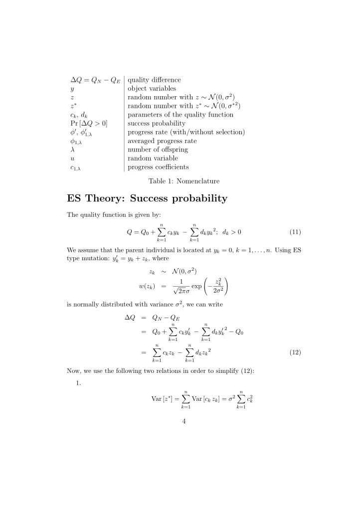
ES Theory: Success probability The quality function is given by: n - PDF document

∆ Q = Q N − Q E quality difference y object variables z random number with z ∼ N (0 , σ 2 ) random number with z ∗ ∼ N (0 , σ ∗ 2 ) z ∗ c k , d k parameters of the quality function Pr [∆ Q > 0] success probability φ ′ , φ ′ progress rate (with/without selection) 1 ,λ φ 1 ,λ averaged progress rate λ number of offspring u random variable c 1 ,λ progress coefficients Table 1: Nomenclature ES Theory: Success probability The quality function is given by: n n � � d k y k 2 ; d k > 0 Q = Q 0 + c k y k − (11) k =1 k =1 We assume that the parent individual is located at y k = 0, k = 1 , . . . , n . Using ES type mutation: y ′ k = y k + z k , where N (0 , σ 2 ) ∼ z k � � − z 2 1 k √ w ( z k ) = 2 πσ exp 2 σ 2 is normally distributed with variance σ 2 , we can write ∆ Q = Q N − Q E n n 2 − Q 0 � � = Q 0 + c k y ′ k − d k y ′ k k =1 k =1 n n � � d k z k 2 = c k z k − (12) k =1 k =1 Now, we use the following two relations in order to simplify (12): 1. n n � Var [ c k z k ] = σ 2 � c 2 Var [ z ∗ ] = k k =1 k =1 4

n σ ∗ 2 = σ 2 � c 2 ⇒ k k =1 � n � σ ∗ = σ � � c 2 ⇒ (13) � k k =1 2. � n � n � d k z 2 = σ 2 � E d k (14) k k =1 k =1 A sum of normally distributed random numbers results in a normally distributed random number with the standard deviation given by equation (13). Therefore, the first term of equation (12) is simply given by z ∗ with z ∗ ∼ N (0 , σ ∗ 2 ). The sum of n normally distributed random numbers with variance one, results for large √ n in the χ 2 -distribution. Since the standard deviation only depends on 2 n , we neglect the “randomness” of the second term and replace it by its average value given in equation (14). Thus, we write n ∆ Q ≈ z ∗ − σ 2 d k ; z ∗ ∼ N (0 , σ ∗ 2 ) � (15) k =1 The probability for success is given by: � n � z ∗ ≥ σ 2 � Pr [∆ Q > 0] = Pr d k k =1 � ∞ � � − z ∗ 2 1 √ dz ∗ = exp (16) 2 σ ∗ 2 2 πσ ∗ σ 2 � d k √ 2 σ ∗ and dz ∗ = 2 σ ∗ dp : z ∗ Now we substitute p = √ √ � ∞ 1 e − p 2 dp √ 2 σ ∗ Pr [∆ Q > 0] = (17) σ 2 � dk 2 πσ ∗ σ ∗√ 2 Using the error function erf ( x ): � x 2 e − p 2 dp, √ π erf( x ) = (18) 0 �� c 2 and σ ∗ = σ k we can write σ �   dk � ∞ 1 e − p 2 dp − e − p 2 dp � � 2 � c 2 Pr [∆ Q > 0] = √ π   k   0 0 5

     σ � n 1 k =1 d k =  1 − erf (19)   2 � 2 � n k =1 c 2 k ES Theory: Progress rate The progress rate φ ′ is defined as follows: φ ′ = ∆ Q (20) tan α, where ∆ Q is given by equation (14). Since tan α is the gradient at the parent position, i.e. at y k = 0; k = 1 , . . . , n , we have � n � ∂Q � n � 1 � 1 � 2 2 2 � � c 2 tan α = = (21) . k ∂y k y k =0 k =1 k =1 Therefore, the progress rate is given by � n z ∗ k =1 d k φ ′ = − σ 2 . (22) � 1 � 1 �� n �� n k =1 c 2 k =1 c 2 2 2 k k Using the following equation � n � n � 1   � n 2 Var [ z ∗ ] = σ 2 � c 2 � c 2 � c 2  , = k Var [ z ] = Var z (23) k  k k =1 k =1 k =1 we can simplify equation (22): � n k =1 d k φ ′ = z − σ 2 (24) . � 1 �� n k =1 c 2 2 k Since the random variable z is symmetric around E [ z ] = 0, we see from equation (24) that a positive progress rate can only be achieved with selection. If we assume (1 , λ ) selection, we have to derive the probability density of a new random variable u , which is the largest out of λ random numbers z i , i = 1 , . . . , λ and z i = N (0 , σ 2 ). Therefore, after selection we have to replace equation (24) by � n k =1 d k 1 ,λ = u − σ 2 φ ′ (25) . � 1 �� n k =1 c 2 2 k 6

If we denote the probability density of u by w λ ( u ), the expectation value of φ ′ 1 ,λ is given by: � ∞ � n k =1 d k � � u w λ ( u ) du − σ 2 φ ′ φ 1 ,λ = E = (26) 1 ,λ � 1 �� n k =1 c 2 −∞ 2 k � n k =1 d k σ c 1 ,λ − σ 2 = , (27) � 1 �� n k =1 c 2 2 k � u � � � 1 − u 2 ��� λ − 1 λ � √ √ w λ = 2 πσ exp 1 + erf (28) 2 σ 2 2 2 σ where we have introduced the progress rate coefficients c 1 ,λ : √ � ∞ 2 λ ze − z 2 [1 + erf( z )] λ − 1 dz √ π 2 λ − 1 c 1 ,λ = (29) −∞ Note, that the formula for the progress rate, equation (27), remains the same even for the more general ( µ, λ ) selection, only the progress rate coefficients change and are replaced by c µ,λ . ES theory: 1 / 5 -rule With the results from the last section, we are now able to determine the step-size that leads to the maximal progress rate: � n ∂φ 1 ,λ k =1 d k ⇒ = 0 c 1 ,λ = 2 σ � 1 ∂σ �� n k =1 c 2 2 k � 1 �� n k =1 c 2 σ opt = c 1 ,λ 2 k ⇒ . (30) � n 2 k =1 d k This corresponds to a progress rate of � 1 �� n k =1 c 2 φ 1 ,λ,opt = 1 2 4 c 2 k (31) 1 ,λ � n k =1 d k At the same time the sucess probability for σ opt is given by     � n 1  σ opt k =1 d k Pr [∆ Q > 0] =  1 − erf   � 2 2 � n k =1 c 2 k � c 1 ,λ 1 � �� √ = 1 − erf . 2 2 2 7