Error-correcting learning: Delta rule Effects of training on - PowerPoint PPT Presentation

Error-correcting learning: Delta rule Effects of training on response to input patterns Important distinction (and notation): Calculated in terms of changes to activations for pattern p ′ caused by training on single t j target of unit j ; the (correct) activation specified by the environment (training example) pattern p: a j activation of unit j that results from actually running the network △ a [p ′ ] a [p ′ ] � = △ w ij j i Note: in Hebb rule, a j was specified and so would now be called t j i a [p ′ ] � t [p] − a [p] � a [p] � Hebb rule: △ w ij = ǫ t j a i (where t j is activation “clamped” on the output unit) = ǫ i j j i i � � � a [p ′ ] Delta rule : Change weights so as to reduce difference between actual output ( a j ) and target t [p] − a [p] a [p] = ǫ j j i i output ( t j ) (“delta” = difference between target and activation) i � � t [p] − a [p] dp (p ′ , p) = ǫ ( t j − a j ) a i = ǫ △ w ij j j Similar to correlation with error If p and p ′ are orthogonal, training on p will have no effect on p ′ If p and p ′ are not orthogonal, training on p will affect performance on p ′ (weighted by Weight changes focus on predictive differences similarity) which may be good (generalization) or bad (interference) Hebbian/correlational learning depends on predictive similarities 1 / 11 3 / 11 Learning on orthogonal patterns (one pass): Delta = Hebb 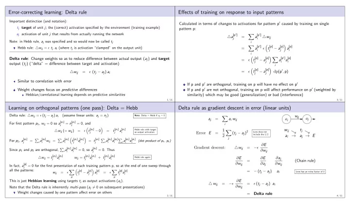Delta rule as gradient descent in error (linear units) Delta rule: △ w ij = ǫ ( t j − a j ) a i (assume linear units: a j = n j ) Note : Delta = Hebb if a j = 0 � a j = a i w ij For first pattern p 1 , w ij = 0 so a [ p 1 ] = n [ p 1 ] = 0, and i j j � � t [ p 1 ] t [ p 1 ] a [ p 1 ] 1 w ij t j Hebb rule with target △ w ij (= w ij ) = ǫ − 0 = � ( t j − a j ) 2 Lens does not j j i as output activation Error E = include the 1/2 2 a i → a j → E j � � For p 2 , a [ p 2 ] i a [ p 2 ] i a [ p 2 ] t [ p 1 ] a [ p 1 ] = t [ p 1 ] i a [ p 2 ] a [ p 1 ] i a [ p 2 ] a [ p 1 ] = � w ij = � � � (dot product of p 1 , p 2 ) j i i j i j i i i i − ǫ ∂ E Gradient descent: △ w ij = i a [ p 2 ] a [ p 1 ] = 0, so a [ p 2 ] Since p 1 and p 2 are orthogonal, � = 0. Thus ∂ w ij i i j △ w ij = t [ p 2 ] a [ p 2 ] w ij = t [ p 1 ] a [ p 1 ] + t [ p 2 ] a [ p 2 ] Hebb rule again ∂ E ∂ E ∂ a j j i j i j i = (Chain rule) ∂ w ij ∂ a j ∂ w ij In fact, a [p] = 0 for the first presentation of each training pattern p, so at the end of one sweep through j all the patterns: � � = − ( t j − a j ) a i � t [p] − a [p] a [p] � t [p] j a [p] w ij = ǫ = ǫ Lens has an extra factor of 2 j j i i p p This is just Hebbian learning using targets t j as output activations ( a j ). − ǫ ∂ E △ w ij = = ǫ ( t j − a j ) a i ∂ w ij Note that the Delta rule is inherrently multi-pass ( a j � = 0 on subsequent presentations) Weight changes caused by one pattern affect error on others = Delta rule 2 / 11 4 / 11

Delta rule as gradient descent in error (sigmoid units) Linear separability � n j = a i w ij Delta rule is guaranteed to succeed at binary classification if the task is linearly separable i 1 a j = 1 + exp ( − n j ) w ij t j Weights define a plane (line for two input units) through 1 a i → n j → a j → E input (state) space for which n j = 0 � ( t j − a j ) 2 = Error E 2 Must be possible to position this plane such that all j patterns requiring n j < 0 are on one side and all patterns − ǫ ∂ E requiring n j > 0 are on the other side = Gradient descent: △ w ij ∂ w ij Property of the relationship between input and target n j = a 1 w 1 + a 2 w 2 + b j = 0 ∂ E ∂ E d a j ∂ n j patterns = a 2 = − w 1 a 1 − b j ∂ w ij ∂ a j d n j ∂ w ij AND and OR are linearly separable but XOR is not w 2 w 2 = − ( t j − a j ) a j (1 − a j ) a i ( y = + b ) a x − ǫ ∂ E △ w ij = = ǫ ( t j − a j ) a j (1 − a j ) a i ∂ w ij 5 / 11 7 / 11 When does the Delta rule succeed or fail? XOR Delta rule is optimal n j = a 1 w 1 + a 2 w 2 + b j = 0 Will find a set of weights that produces zero error if such a set exists a 2 = − w 1 a 1 − b j w 2 w 2 ( y = + b ) a x Need to distinguish “succeed” = zero error from “succeed” = correct binary classification Guaranteed to succeed (zero error) if input patterns are linearly independent (LI) No pattern can be created by recombining scaled versions of the others (i.e., there is something unique about each pattern; cf. Hebb: no similarity) Orthogonal patterns are linearly independent (LI is a weaker constraint) Linearly independent patterns can be similar as long as other aspects are unique Succeed at binary classification of outputs: Linear separability 6 / 11 8 / 11

XOR with extra dimension XOR task can be converted to one that is linearly separable by adding a new “input” Corresponds to a third dimension in state space Task is no longer XOR Inputs Output 0 0 0 0 0 1 0 1 1 0 0 1 1 1 1 0 9 / 11 11 / 11 XOR with intermediate (“hidden”) units Intermediate units can re-represent input patterns as new patterns with altered similarities Targets which are not linearly separable in the input space can be linearly separable in the intermediate representational space Intermediate units are called “hidden” because their activations are not determined directly by the training environment (inputs and targets) 10 / 11