Error analysys When we make a measurement, we generally assume that - PowerPoint PPT Presentation

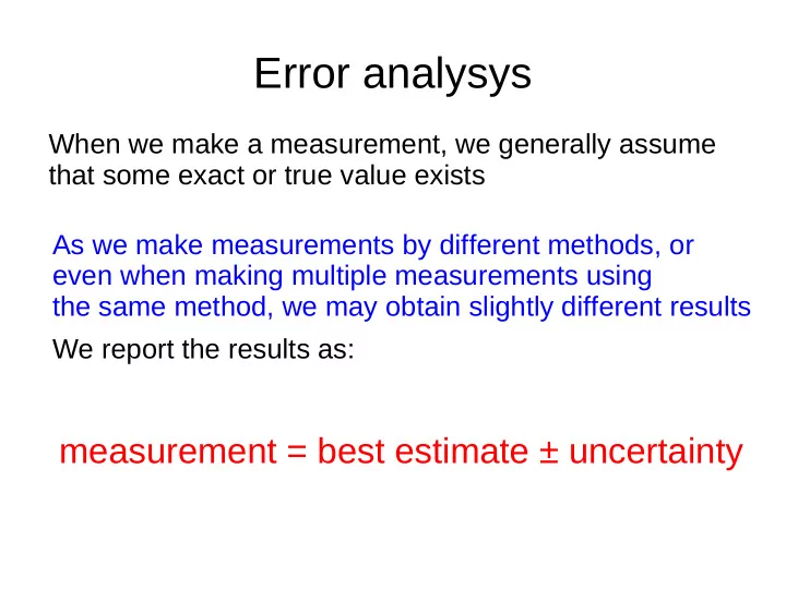
Error analysys When we make a measurement, we generally assume that some exact or true value exists As we make measurements by different methods, or even when making multiple measurements using the same method, we may obtain slightly different results We report the results as: measurement = best estimate ± uncertainty

Statistically the Same ● Student A = 30 ± 2 ● Student B = 34 ± 5 ● Since the uncertainties for A & B overlap, these numbers are statistically the same

Accuracy and precision Accuracy is the closeness of agreement between a measured value and a true or accepted value. Measurement error is the amount of inaccuracy. Precision is a measure of how well a result can be determined (without reference to a theoretical or true value). It is the degree of consistency and agreement among independent measurements of the same quantity; also the reliability or reproducibility of the result.

Accuracy Accuracy is often reported quantitatively by using relative error: Note that the fractional uncertainty is dimensionless (the uncertainty in cm was divided by the average in cm). An experimental physicist might make the statement that this measurement "is good to about 1 part in 500" or "precise to about 0.2%"

Precision Precision is often reported quantitatively by using relative or fractional uncertainty:

Types of error Random errors are statistical fluctuations (in either direction) in the measured data due to the precision limitations of the measurement device. Random errors can be evaluated through statistical analysis and can be reduced by averaging over a large number of observations (see standard error). Systematic errors are reproducible inaccuracies that are consistently in the same direction. These errors are difficult to detect and cannot be analyzed statistically. If a systematic error is identified when calibrating against a standard, the bias can be reduced by applying a correction or correction factor to compensate for the effect. Unlike random errors, systematic errors cannot be detected or reduced by increasing the number of observations. Our strategy is to reduce as many sources of error as we can, and then to keep track of those errors that we can't eliminate. It is useful to study the types of errors that may occur, so that we may recognize them when they arise.

Common sources of error Incomplete definition: clearly define the measurement conditions (environment, ● instruments) – systematic or random Failure to account for a factor: consider all factors that could affect the ● measurement: gravity, resistance of air, nearby electromagnetic fields... systematic Environmental conditions: vibrations, drafts, changes in temperature, electronic ● noise or other effects from nearby apparatus – systematic or random Instrument resolution: random ● Failure to calibrate or check zero of instrument: - systematic ● Parallax : This error can occur whenever there is some distance between the ● measuring scale and the indicator used to obtain a measurement. If the observer's eye is not squarely aligned with the pointer and scale, the reading may be too high or low (some analog meters have mirrors to help with this alignment). – systematic or random Instrument drift: Most electronic instruments have readings that drift over time – ● systematic Lag time and hysteresis : Some measuring devices require time to reach ● equilibrium, and taking a measurement before the instrument is stable will result in a measurement that is generally too low – systematic

Uncertainty for a Single Measurement The uncertainty of a single measurement is limited by the precision and accuracy of the measuring instrument, along with any other factors that might affect the ability of the experimenter to make the measurement. Example: Single measurement with a ruler Sources of error: a) instrument resolution b) positioning c) parallax Uncertainty of a single measurement: add up the three

Uncertainty in Repeated Measurements Whenever possible, repeat a measurement several times and average the results. This average is the best estimate of the "true" value. The more repetitions you make of a measurement, the better this estimate will be.

Standard deviation To calculate the standard deviation for a sample of N measurements: 1. Sum all the measurements and divide by N to get the average or mean. 2. Now, subtract this average from each of the N measurements to obtain N "deviations". 3. Square each of these N deviations and add them all up. 4. Divide this result by N-1, and take the square root. We can write out the formula for the standard deviation as follows. Let the N measurements be called x1, x2,..., xN. Let the average of the N values be called x. Then each deviation is given by

Standard Deviation of the Mean (Standard Error) When we report the average value of N measurements, the uncertainty we should associate with this average value is the standard deviation of the mean, often called the standard error (SE). This reflects the fact that we expect the uncertainty of the average value to get smaller when we use a larger number of measurements N

Example Meas. # Value (cm) 1 405 2 404 3 403 4 402 5 405 X=1/5(405+404+403+402+405)=403.8 σ 2 =1/20(1.44+0.04+0.64+3.24+1.44)=0.34 σ =0.58 X=403.8 ± 0.6

Anomalous data Anomalous data points that lie outside the general trend of the data may suggest an interesting phenomenon that could lead to a new discovery, or they may simply be the result of a mistake or random fluctuations. Require closer examination to determine the cause of the unexpected result. Extreme data should never be "thrown out" without clear justification and explanation

Propagation of uncertainty Examples: a) f = x+y b) f = x.y (same for division)

Significant figures The number of significant figures in a value can be defined as all the digits between and including the first non-zero digit from the left, through the last digit. For multiplication and division, the number of significant figures that are reliably known in a product or quotient is the same as the smallest number of significant figures in any of the original numbers. Example: 6.6 (2 significant figures) x 7328.7 (5 significant figures) 48369.42 = 48 x 10 3 (2 significant figures) For addition and subtraction, the result should be rounded off to the last decimal place reported for the least precise number. Examples: 223.64 5560.5 +54 +0.008 278 5560.5 If a calculated number is to be used in further calculations, it is good practice to keep one extra digit to reduce rounding errors that may accumulate. Then the final answer should be rounded according to the above guidelines.

Uncertainty and significant figures For the same reason that it is dishonest to report a result with more significant figures than are reliably known, the uncertainty value should also not be reported with excessive precision. For example, if we measure the density of copper, it would be unreasonable to report a result like: measured density = 8.93 ± 0.4753 g/cm3 WRONG!

Basic recipe The uncertainty should be rounded off to one or two significant figures. If the leading figure in the uncertainty is a 1, we use two significant figures, otherwise we use one significant figure. Then the answer should be rounded to match the same number of digits (or decimal places) In the previous example: measured density = 8.9 ± 0.5 g/cm3 RIGHT! We always overestimate the error, so we round off upwards. Never underestimate the errors!

Example 1 w = (4.52 ± 0.02) cm, x = ( 2.0 ± 0.2) cm, y = (3.0 ± 0.6) cm. Find z = x + y - w and its uncertainty. Solution: z = x + y - w = 2.0 + 3.0 - 4.5 = 0.5 cm ∆ z = 0.633 cm z = (0.5 ± 0.6) cm

Example 2 The radius of a circle is x = (3.0 ± 0.2) cm. Find the circumference and its uncertainty. Solution: C = 2 p x = 18.850 cm ∆ C = 2 p ∆ x = 1.257 cm (The factors of 2 and p are exact) C = (18.8 ± 1.3) cm We round the uncertainty to two figures since it starts with a 1, and round the answer to match the number of decimal places. For multiplication by an exact number, multiply the uncertainty by the same exact number.

Example 3 w = (4.52 ± 0.02) cm, x = (2.0 ± 0.2) cm. Find z = w x and its uncertainty. Solution: z = w x = (4.52) (2.0) = 9.04 ∆ z = 0.905 and z = (9.0 ± 0.9). The uncertainty is rounded to one significant figure and the result is rounded to match the number of decimal places. We write 9.0 rather than 9 since the 0 is significant.