
SLIDE 1
Error analysis
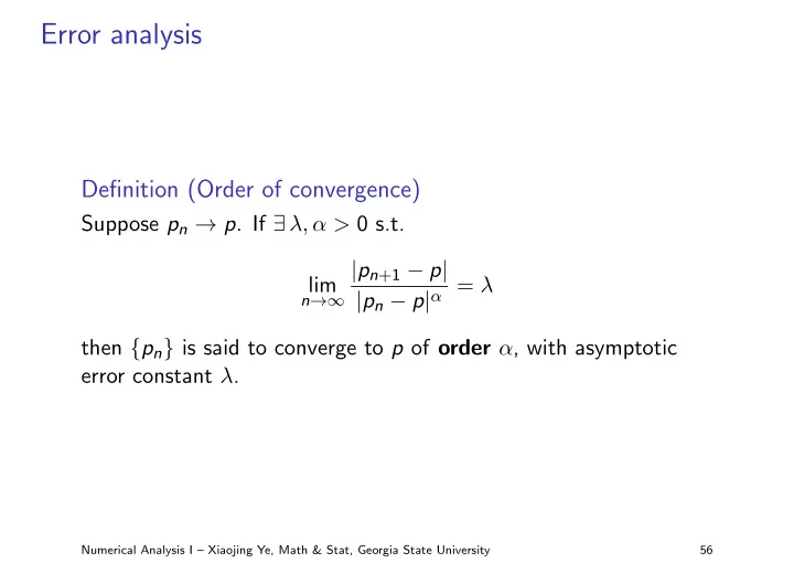
Definition (Order of convergence)
Suppose pn → p. If ∃ λ, α > 0 s.t. lim
n→∞
|pn+1 − p| |pn − p|α = λ then {pn} is said to converge to p of order α, with asymptotic error constant λ.
Numerical Analysis I – Xiaojing Ye, Math & Stat, Georgia State University 56