EQUALITY IN TABLEAUX 13ai In developing a tableau involving - - PowerPoint PPT Presentation

AUTOMATED REASONING SLIDES 13: EQUALITY IN TABLEAUX Basic use of Equality in Tableaux Use of Equality in ME

KB - AR - 13 13ai

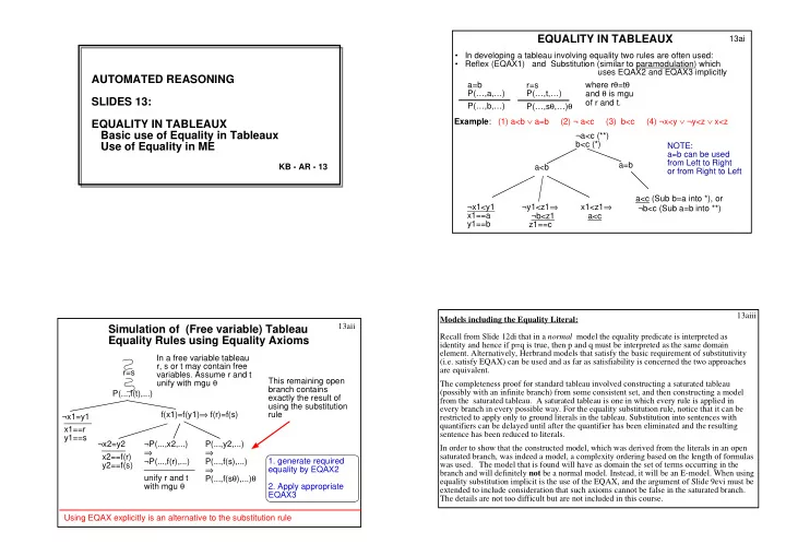
• In developing a tableau involving equality two rules are often used:
• Reflex (EQAX1) and Substitution (similar to paramodulation) which

uses EQAX2 and EQAX3 implicitly a=b P(…,a,…) P(…,b,…) r=s P(…,t,…) P(…,sθ,…)θ where rθ=tθ and θ is mgu

• f r and t.

EQUALITY IN TABLEAUX

Example: (1) a<b ∨ a=b (2) ¬ a<c (3) b<c (4) ¬x<y ∨ ¬y<z ∨ x<z a<b a=b ¬x1<y1 x1==a y1==b ¬y1<z1⇒ ¬b<z1 z1==c x1<z1⇒ a<c a<c (Sub b=a into *), or ¬b<c (Sub a=b into **) ¬a<c (**) b<c (*) NOTE: a=b can be used from Left to Right

• r from Right to Left

13aii

Simulation of (Free variable) Tableau Equality Rules using Equality Axioms

r=s P(...,f(t),...) ¬x1=y1 f(x1)=f(y1)⇒ f(r)=f(s) ¬x2=y2 ¬P(...,x2,...) ⇒ ¬P(...,f(r),...) P(...,y2,...) ⇒ P(...,f(s),...) ⇒ P(...,f(sθ),...)θ x1==r y1==s x2==f(r) y2==f(s) unify r and t with mgu θ This remaining open branch contains exactly the result of using the substitution rule In a free variable tableau r, s or t may contain free

• variables. Assume r and t

unify with mgu θ

• 1. generate required

equality by EQAX2

• 2. Apply appropriate

EQAX3 Using EQAX explicitly is an alternative to the substitution rule 13aiii Models including the Equality Literal: Recall from Slide 12di that in a normal model the equality predicate is interpreted as identity and hence if p=q is true, then p and q must be interpreted as the same domain

• element. Alternatively, Herbrand models that satisfy the basic requirement of substitutivity

(i.e. satisfy EQAX) can be used and as far as satisfiability is concerned the two approaches are equivalent. The completeness proof for standard tableau involved constructing a saturated tableau (possibly with an infinite branch) from some consistent set, and then constructing a model from the saturated tableau. A saturated tableau is one in which every rule is applied in every branch in every possible way. For the equality substitution rule, notice that it can be restricted to apply only to ground literals in the tableau. Substitution into sentences with quantifiers can be delayed until after the quantifier has been eliminated and the resulting sentence has been reduced to literals. In order to show that the constructed model, which was derived from the literals in an open saturated branch, was indeed a model, a complexity ordering based on the length of formulas was used. The model that is found will have as domain the set of terms occurring in the branch and will definitely not be a normal model. Instead, it will be an E-model. When using equality substitution implicit is the use of the EQAX, and the argument of Slide 9evi must be extended to include consideration that such axioms cannot be false in the saturated branch. The details are not too difficult but are not included in this course.

Controlling Equality Substitution in Tableaux: There have been several methods proposed for controlling the use of equality in (free variable)

• tableaux. Many involve the separation of the equality reasoning from standard rules in some

way or other. A simple method is shown on 13bii. Here, a tableau is developed to a maximum depth, closing branches in the usual way if possible. If open branches remain, which also contain equations, an attempt is made to find a contradiction using the equations. Potential closure between 2 literals is made, subject to the constraint that the arguments can be made

• equal. e.g. P(a,f(X)) and ¬P(b, g(b)) would be complementary, if a=b and g(b)=f(X) (for some

X) could be derived. (This is quite similar to the RUE refinement.) The contradiction can be derived in many ways; e.g. a refutation by resolution and substitution (paramodulation) using the equations E in the branch in which closure from E+{¬a=b}+ {¬g(b)=f(X)} is derived. There are several other approaches, but there isn't time to consider most of them here. Instead, remember that on Slide 13aii we showed that using equations in tableaux can be simulated using the equality axioms. Hence an approach to their control would be to incorporate this simulation within the strategy used to develop the tableau. We'll look at just one such strategy, in which a RUE style of using the Alternative EQAX is introduced into clausal ME tableau. It's also possible to use the EQAX in the ME tableau style - see Optional material for Slides 13. 13bi 13bii Here's one possible method:

• Form a tableau to some limit

(eg allow each universal rule to be expanded once and then allow a maximum number of “extra” applications.)

• Ignore substitution using equality

literals, but allow those branches that can close in the usual way to do so.

• For each unclosed branch apply

equality rules to the equations in it in

• rder to force a closure (see

example on right). P(a) ¬P(b) Q(u1,f(b)) ¬Q(c,g(b)) b=c f(c)=g(c) Branch will close if can show (a=b) ∨ (u1=c & f(b)=g(b)) b=c (equalities from f(c)=g(c) branch) a≠b (from negated goal) u1≠c ∨ f(b)≠g(b) (from negated goal) Close? Yes, if u1==b The most difficult aspect of dealing with equality is in controlling substitution as there are usually numerous ways to apply it in a tableau branch.

Controlling Equality Substitution in Tableaux EXAMPLE 1

13biii a) Use each non-unit clause a maximum of once in each branch (assume this is the limit) b) Can close first branch normally by unification c) Can close at (**) if f(g(b))=g(g(w1)) is shown If z1==g(b) and w1==b, can show f(g(b))=g(g(w1)) by Sub with g(z1)=f(z1) More systematically, required to refute ¬(f(g(b))=g(g(w1))) Use Sub with f(z1)=g(z1) to give ¬(g(g(b))=g(g(w1))), binding z1==g(b) Then close with x=x, binding w1==b (**) Q(y1) ¬P(f(y1)) y1==g(b) ⇒ ¬P(f(g(b))) (unify) ¬Q(g(b)) g(z1)=f(z1) P(g(g(w1))) Given: ¬Q(g(b)) Q(y) ∨ ¬P(f(y)) g(z)=f(z) P(g(g(w)))

Given: x=a ∨ x=b g(x)≠g(y) ∨ x=y g(a)=b g(g(a))≠a

EXAMPLE 2 (see ppt)

13biv a) Use each non-unit clause a maximum of once in each branch (the limit). b) Can close first branch normally by unification (match with g(g(a))≠a). c) Can close at (*) if g(y2)=b is shown and either x2==g(a) (match with g(g(a))=b),

• r x2==a (match with g(a)=b)

To show g(y2)=b, set y2==g(a) or y2==a; unify x2; Together, the bindings for x2 and y2 give 4 possibilities for (**): di) y2==g(a), x2==g(a): cannot refute g(a)=g(a). dii) y2==g(a), x2==a: ==> refute a=g(a) (see (e) on slide 13bv) diii) y2==a, x2==a: cannot refute a=a. div) y2==a, x2==g(a): ==> refute g(a)=a (see (e) on slide 13bv) x2=y2 (**) x1=a x1=b x1==g(g(a)) ⇒ g(g(a))=b g(x2)≠g(y2) (*) (unify) g(a)=b g(g(a))≠a

EXAMPLE continued

13bv x2=y2 =>g(a) = a (**) x1=b⇒ g(g(a))=b g(a)=b g(g(a))≠a e) From 13biv one remaining branch (**) to close: Can close if either: g(g(a))=g(a) can be shown (match g(a)=a with g(g(a))≠a),

• r: a=b can be shown

(match g(g(a))=b with g(g(a))≠a) See steps below – add to equations either g(g(a))≠g(a) or a≠b

• 1. g(g(a))≠g(a)
• 2. g(a)=b
• 3. g(g(a))=b
• 4. g(a)=a

g(a)≠g(a) (1+4) close by reflex b≠g(a) (1+3) close by (2) either:

• 1. a≠b
• 2. g(a)=b
• 3. g(g(a))=b
• 4. g(a)=a

g(a)≠b (1+4) close by (2) Using Method of Slide 13bii in Tableaux: The examples on 13biii - 13bv illustrate the method of forming a tableau to some limit (here using each clause a maximum of once in each branch) and then trying to close branches using

• equations. In the first example on 13biii, each clause is used once in a free variable tableau. One

branch closes normally with the unifier y1==g(b). The second branch will close if f(g(b)) and g(g(z1)) can be shown to be equal. In the second example, there are two open branches and two possible closures for the first of these: between g(a)=b and g(x2)≠g(y2), or between g(g(a))=b and g(x2)≠g(y2). One can obtain closure either if x2==a and g(y2)=b can be derived, or if x2==g(a) and g(y2)=b can be derived. i.e. refute ¬g(y2)=b using the set of equations {g(a)=b, g(g(a))=b}, which is easy: y2==a or y2==g(a). There is another possibility, to close g(x2)=g(y2) by reflex, but this yields x2=x2 in the second open branch which cannot be refuted. For the second open branch, two of the substitution pairs result in a=a or g(a)=g(a), which clearly cannot be refuted as they are instances of (Reflex). The other two substitution pairs both result in g(a)=a and the branch can be closed if g(g(a))≠a matches either g(g(a))=b, or g(a)=a or g(a)=b. The first of these requires b=a to be shown using {g(a)=a, g(a)=b}, which is clearly possible; the second requires g(g(a))=g(a) to be shown, again using {g(a)=a, g(a)=b}. Again this is easy. The third requires to show g(g(a))=g(a) and a=b, which is done as before. (See 13bv for some of the cases.) Only one of these options is necessary. Exercise: Show these things. 13bvi It is clear from these exemplars that there are many and various possibilities when using equations and that the search space can become very large.

EXAMPLE 3 13ci ME tableau with equality - implicit EQAX RUE style Remember - can use symmetry (1) here the match can be a normal closure (2) try to match P(f(g(b))) with P(g(g(w1))); results in requiring to show g(g(w1))=f(g(b)) (3) try to match g(g(w1))=f(g(b)) with g(z1)=f(z1); need to show both g(w1)=z1, and g(b)=z1. The first binds z1==g(w1) and the second then binds w1==b. Note: Resolution steps with EQAX1 and EQAX2 are made implicitly. eg at (3) RUE-style gives g(w1)≠z1 as well as g(b)≠z1. There are still many different possibilities for closure: Q: Give a tableau that could result if the top clause literal order was reversed? Given: ¬Q(g(b)), Q(y) ∨ ¬P(f(y)) g(z)=f(z), P(g(g(w))) Q(y1) y1==g(b) (1) ¬P(f(y1)) => ¬P(f(g(b))) g(g(w1))≠f(g(b)) ¬Q(g(b)) g(b)≠z1 ==>g(b)≠g(w1) P(g(g(w1))) g(z1)=f(z1) g(w1)≠z1 z1==g(w1) (2) w1==b (3) Given: x=a ∨ x=b g(g(a))≠a g(a)=b g(x)≠g(y) ∨ x=y EXAMPLE 4 13cii ME tableau with equality - RUE style Another example: (1) here try to match g(x1)≠g(y1) with g(g(a))=b; results in need to show b=g(y1) as in branch at (2) (2) follows by a normal closure (remember can use symmetry) (3) try to match g(a)=a with g(g(a))≠a; results in need to show g(g(a))=g(a) (ie literal g(g(a))≠g(a) (4) try to match g(g(a))≠g(a) with g(g(a))=b; results in need to show g(a)=b, which results in literal g(a)≠b which closes normally. Can you find a different tableau? x2=a x2==g(g(a)) x2=b => g(g(a))=b (3) g(g(a))≠g(a) g(x1)≠g(y1) x1==g(a) (1) b≠g(y1) (2) x1=y1==> g(a)=y1==> g(a)=a g(a)≠b (4) g(g(a))≠a g(a)=b y1==a g(a)=b 13ciii Using EQAX implicitly in Model Elimination Tableaux: Slides 13ci and 13cii show tableaux in which EQAX are used implicitly in Model Elimination to simulate a RUE style. The axioms used are particular for the predicate(s) involved, which may even be the equality predicate itself. In that case the axioms are ¬x=y ∨ g(x)=g(y), ¬x=w ∨ ¬y=z ∨ ¬x=y ∨ w=z The first axiom is an instance of EQAX2 and the second is an instance of (Alt) EQAX3, where "P" of the axiom is the "=" predicate (c.f. ¬x=w ∨ ¬y=z ∨ ¬P(x,y) ∨ ¬P(w,z)). Use of the reflexive EQAX1 (x=x) is often needed. Symmetry can be built in; e.g. unifying (say) a=b with ¬x1=x2, results in two unifiers: {x1==a, x2==b} and {x1==b,x2==a}. The implicit use of the Axioms is made by matching two literals with the same predicate. To match P(x,y) with ¬P(u,v), for example, the closure would be made, but additional branches with the leaves ¬x=y and ¬u=v would be added. For example, this happens in several places on 13cii, namely at closures (2), (3) and (4). At (2) it arises due to matching g(g(a))=b in the tableau branch with g(x1)≠g(y1) from the clause x=y ∨ ¬g(x)=g(y). The additional inequality is b≠g(y1). At (3) it arises due to matching g(a)=a with g(g(a))≠a. At (4) it arises due to matching g(g(a))≠g(a) with g(g(a))=b. 13di

Summary of Slides 13

• 1. Equality reasoning can be incorporated into tableau, either standard tableau,

free variable tableau or ME tableau.

• 2. In standard tableau the equality rule allows to derive new ground literals using

equality substitution; in free variable tableau it allows to derive new literals, possibly applying a unifying substitution (also called paramodulation).

• 3. Usually, a tableau is developed to some depth, closing branches normally if

possible, and then attempting to close remaining branches using any equalities in the branch.

• 4. Most methods using equality in tableau are quite difficult for humans to carry out

and lead to large seach spaces.

• 5. Use of the equality axioms can be simulated within ME tableau, by using equality

axioms implicitly (shown for the RUE approach).

• 6. Use of EQAX can also be used in ME style explicitly to simulate the RUE

approach (see optional material), or paramodulation (not shown here).

S ST TA AR RT T

• f

f O OP PT TI IO ON NA AL L M MA AT TE ER RI IA AL L ( (S SL LI ID DE ES S 1 13 3) )

Using EQAX explicitly

13ei Using EQAX explicitly in Model Elimination Tableaux: Slide 13eii shows a tableau in which EQAX are used explicitly in Model Elimination to simulate a RUE style. As before, the axioms used are particular for the predicate(s) involved. Various restrictions could be incorporated into the use of these axioms. For instance, the use

• f EQAX could be restricted to use in a branch B such that at most one literal remains
• unclosed. Closure could either be with a literal in B, or with a fact. This restriction could

simulate both paramodulation and RUE, in different circumstances. For example, in the EQAX3, ¬x1=x2 ∨ ¬y1=y2 ∨ ¬P(x1,y1) ∨ P(x2,y2), if either ¬x1=x2 or ¬y1=y2 remained unclosed, this would be a RUE type step, whereas if ¬P(x1,y1) or P(x2,y2) remained unclosed it would be a paramodulation type step (Check this). Other restrictions were investigated by Rosa Gutierrez-Escudero in 2010 (available as a distinguished project on the doc website). Unfortunately, the above restriction is not complete (can you find a counterexample?). Slide 13eii uses the restriction. Notice at most one literal in a clause is extended; all the others close immediately. It is also possible to use the equality axioms explicitly to simulate paramodulation in a ME

• tableau. Alternatively, the equality axioms can be added as input clauses and standard ME

rules applied, not trying to simulate any particular strategy. If combined with other strategies, such as pruning non-essential backtracking and the GCR, this can often be the best option. It is also the simplest to implement. The drawback, compared with implicit use of EQAX, is that all the necessary axioms must be added at the start. Given: x=a ∨ x=b g(g(a))≠a g(x)≠g(y) ∨ x=y g(a)=b ¬x=u ∨ ¬y=v ∨ ¬x=y ∨ u=v (Alt EQAX3) x=x (EQAX1) 13eii ME tableau with explicit EQAX - RUE style this clause is an EQAX3 used to simulate the RUE step of matching g(g(a))=b with g(x3)≠g(y3) (see ii) Can use symmetry at (i) again use an EQAX to simulate RUE step of matching g(a)=a with ¬g(g(a))=a. Because the EQAX are explicit, there is direct closure with u2=v2 ==> g(g(a))=g(a) (see iii) EXAMPLE 5 x1=a x1==g(g(a)) x1=b => g(g(a))=b g(x3)≠g(y3) u2==g(x3) v2==g(y3) (ii) g(a)=b g(g(a))≠a ¬x4=y4 x4==g(a) y4==a ¬x4=u4 ==> ¬g(a)=g(g(a)) (iii) x3=y3 ==> g(a)=a u4=v4 u4==g(g(a)) v4==a ¬x2=y2 x2==g(g(a)) y2==b u2=v2 ¬x2=u2==> ¬g(g(a))=u2==> ¬g(g(a))=g(x3) x3==g(a) (use EQAX1) ¬y2=v2 ¬b=g(y3) y3==a (i) ¬y4=v4 ==> ¬a=a