Clausal Tableaux and Linear Strategies Clausal Tableaux use only - - PowerPoint PPT Presentation

AUTOMATED REASONING SLIDES 10: CLAUSAL TABLEAUX Model Elimination Short-cuts: Lemmas and Merging

KB - AR - 13 10ai

• Clausal Tableaux use only clausal sentences
• Clause Extension rule is derived from free variable γ-rule and ∨-splitting.

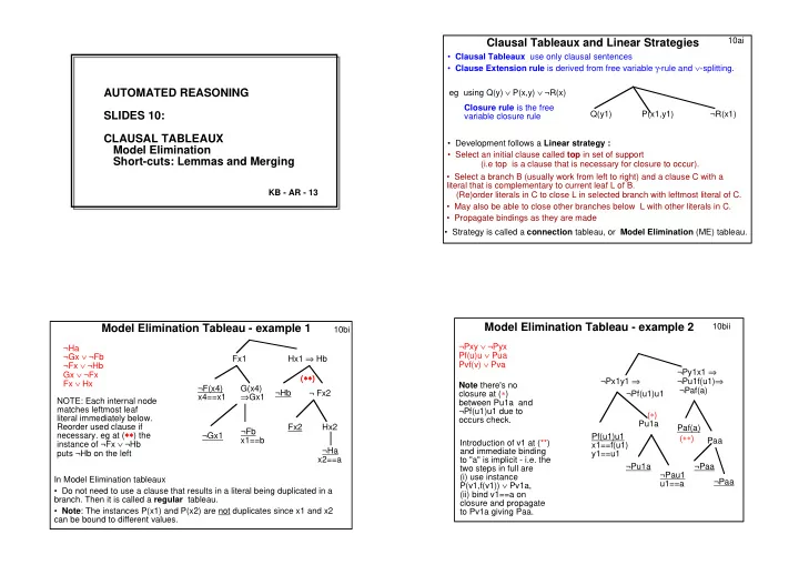
Clausal Tableaux and Linear Strategies

Q(y1) P(x1,y1) ¬R(x1)

• Development follows a Linear strategy :
• Select an initial clause called top in set of support

(i.e top is a clause that is necessary for closure to occur). Closure rule is the free variable closure rule eg using Q(y) ∨ P(x,y) ∨ ¬R(x)

• Strategy is called a connection tableau, or Model Elimination (ME) tableau.
• Select a branch B (usually work from left to right) and a clause C with a

literal that is complementary to current leaf L of B. (Re)order literals in C to close L in selected branch with leftmost literal of C.

• May also be able to close other branches below L with other literals in C.
• Propagate bindings as they are made

10bi NOTE: Each internal node matches leftmost leaf literal immediately below. Reorder used clause if

• necessary. eg at (∗

∗ ∗ ∗∗ ∗ ∗ ∗) the instance of ¬Fx ∨ ¬Hb puts ¬Hb on the left

Model Elimination Tableau - example 1

¬Ha ¬Gx ∨ ¬Fb ¬Fx ∨ ¬Hb Gx ∨ ¬Fx Fx ∨ Hx ¬F(x4) x4==x1 Fx1 Hx1 ⇒ Hb G(x4) ⇒Gx1 ¬Hb ¬ Fx2 ¬Gx1 Fx2 Hx2 ¬Fb x1==b ¬Ha x2==a (∗ ∗ ∗ ∗∗ ∗ ∗ ∗) In Model Elimination tableaux

• Do not need to use a clause that results in a literal being duplicated in a
• branch. Then it is called a regular tableau.
• Note: The instances P(x1) and P(x2) are not duplicates since x1 and x2

can be bound to different values. 10bii ¬Pxy ∨ ¬Pyx Pf(u)u ∨ Pua Pvf(v) ∨ Pva Note there's no closure at (∗) between Pu1a and ¬Pf(u1)u1 due to

• ccurs check.

Model Elimination Tableau - example 2

Introduction of v1 at (**) and immediate binding to "a" is implicit - i.e. the two steps in full are (i) use instance P(v1,f(v1)) ∨ Pv1a, (ii) bind v1==a on closure and propagate to Pv1a giving Paa. ¬Px1y1 ⇒ ¬Py1x1 ⇒ ¬Pu1f(u1)⇒ ¬Paf(a) Pf(u1)u1 x1==f(u1) y1==u1 Pu1a ¬Pu1a ¬Pau1 u1==a ¬Pf(u1)u1 Paf(a) Paa ¬Paa ¬Paa (∗) (∗∗)

10biii Model Elimination Tableaux: The examples of Model Elimination tableaux shown on 10bi/10bii illustrate several features of connection tableaux. On 10bi notice that in the extension below Fx1 an explicit introduction of x4 for x in the use of the clause ¬Fx ∨ Gx is made. The resulting literal ¬Fx4 is matched with Fx1 to give closure with binding (x4==x1). This binding is then propagated through the tableau (indicated by ⇒). These steps can be combined, and in subsequent steps are, to save unnecesary introduction of new free variables. Thus in the next step, below Gx1, a copy of ¬Gx ∨ Fb is taken, implicitly using new free variable x3, to enable closure between ¬Gx3 and Gx1; x3 is immediately bound to x1 and only the value after closure is shown. This saves some clutter in depicting the tableau. Note also the reordering of the instance ¬Fx2 ∨ ¬Hb of ¬Fx ∨ ¬Hb so the leftmost branch closes below Hb. In the example on 10bii the introduction of fresh variable u1 in the first step is made explicit, so the copy (of Pf(u)u ∨ Pua) uses free variable u1. This is reasonable here, as it is the older variable x1 that is bound (x1==f(u1)), not the new one, u1. The bindings must be propagated in the tableau, so ¬Px1y1 becomes ¬Pf(u1)u1 and ¬Py1x1 becomes ¬Pu1f(u1). (Actually, since y1 is also bound to u1, it isn't necessary to introduce u1 here either, since an implicit u1 could be bound to y1 leading to x1==f(y1). However, it is clearer to introduce u1, I think.) Notice that the possible closure between ¬P(x1,y1) ⇒ ¬Pf(u1)u1 and Pu1a fails. When u1 is later bound to a this binding is propagated through to ¬Pu1f(u1) ⇒ ¬Paf(a). Closing a branch by unifying the leaf with a literal higher in the same branch (eg beneath ¬Pau1) hais sometimes been called ancestor closure. 10ci The refutation X (found beneath the rightmost occurrence of ¬B) could also be used below the occurrence at ¬B*. Why? This step is valid only because the tableau is developed left to right; all ancestors of ¬B (indicated by (A)) are available also to ¬B*. On encountering ¬B* and noticing that ¬B occurs also to the right in the ME tableau, can close ¬B* by merging. Merging is the tableau version of factoring.

The Merge Short cut (ground case)

¬M ¬B M L ¬L M ¬B* X X

}A

10cii

Refinements of Model Elimination: There are two simple refinements for ME-tableaux shown on slides 10c, which are here called merging and re-use. Consider the case for propositional tableau first. Important Note 1: merging and re-use cannot both be used in a single tableau; otherwise soundness is not in general maintained. Important Note 2: merging and re-use are only available for ME-tableau; they are possible

• nly because of the left to right development of such tableaux.

Merging is the simplest of the two refinements. If a leaf literal L can be unified with another leaf literal L' in an open branch to its right (necessarily a sibling of L or a sibling of an ancestor of L), then the branch ending at L can be closed by merge without further steps. This is sound because when the (necessary) closure beneath L' is made, it can be repeated (retrospectively) beneath L. Any ancestors needed for the closure beneath L' will also be available beneath L, due to the tableau structure. Merging is the tableau version of factoring. The other extension is called Re-use. If a sub-tableau beneath a literal L at node n closes, then any other occurrences of L at nodes n' that may (later) occur in open branches of the tableau can be closed also, as long as the ancestors needed to close L at n are also available at n'. If the subsequent occurrences of L appear at siblings of n or at descendants of siblings of n, then this will be so. Otherwise, it needs to be checked. In the simplest case, when no ancestors are needed, then any occurrence of L can be closed in the same manner as the occurrence of L at n is closed. The (re-use) rule can be implemented in a simple way by adding the literal ¬L to all branches that are known to share the necessary ancestors. Then closure can be made by the normal closure rule. Usually, implementations consider just 2 cases: when L at n' occurs in a sibling branch and when no ancestors are used to close L at n. 10ciii In the tableau shown the second occurrence of ¬B

• ccurs in the right hand branch at ¬B**, but below

the sibling ¬M of ¬B*. Hence when ¬B* is being extended merge is not an available option. Instead, can apply Re-use: once a closure below a literal has been found (eg closure Y below ¬B*), any other occurrences of that literal can use the same closure (as long as the necessary ancestors are available). eg1 Can use closure Y below ¬B**. Can simulate this by adding the negation of ¬B (ie B) in the branch of ¬B** to represent there has been closure below ¬B*, so when ¬B** is encountered can use closure rule. eg2 Similarly, can use (¬L) to represent closure beneath L in the 3rd branch. This is allowed since the ancestor of L used in the closure beneath it is ¬M, and ¬M is also in the 4th branch.

The Re-use Short cut (Ground case)

¬B* Y ¬M M L ¬B** ¬L M (B) (¬L)

10civ K L ¬L S ¬K S* ¬S ¬K T ¬T S (¬S) (¬K) After closing occurrence of S at S*, notice that ancestor K was

• necessary. Since K is not an

ancestor of S in the right-most branch, cannot re-use here the closure made under S*. Example showing when re-use is NOT applicable Cannot apply re-use to S here In general, re-use is usually used in two cases only: (i) when no ancestors were required in closure beneath a literal (eg case of K in first branch), or (ii) when the second closure is beneath a sibling branch of the first closure (eg case of S* in second branch) Merging in First Order Tableaux: Assume the first occurrence (the one to be closed by merge) is L and that it is to be merged with a second occurrence L' (to its right in the tableau). There are 2 basic cases to consider. Case 1 is when bindings are required to be made to L but not to L'. This case is safe as long as the variables in L that are bound do not occur in other leaf literals in branches to the right of L or in ancestors of L. The reason for the proviso is that the bindings would be propagated to those literals and they may not be appropriate to completing the tableau beneath them. This restricted case is sound because when the (necessary) closure beneath L' is made, it can be repeated beneath L, for after unification they are identical. Any ancestors needed for the closure beneath L' will also be available beneath L, due to the tableau structure. (In fact, if the bindings affect only L and ancestors of L, then the merge is also safe. See Slides 11 for a short discussion of this case). Case 2 is when bindings are required to be made to L'. This case is not usually implemented (see Slide 10dii for an illustration). Exercise: try to construct a simple exemplar for the different cases. 10di 10dii Merging is the tableau version of factoring. In the first order case, analogous to safe factoring, merging is usually restricted s.t. variables in A and ¬B** (and in any other unclosed branches to the right of ¬B* - eg in the branch with ¬M and L) are not bound by the merge step unifier. Variables in ¬B* may be bound.

The Merge Short cut (first order) (1)

¬M ¬B** M L ¬B* X X

}A

eg1: if ¬B* is ¬G(a) and ¬B** is ¬G(x1) then merging binds x1==a. Now, it may be that ¬G(a) can be closed at ¬B* (perhaps using ancestors such as ¬M in the diagram) but not at ¬B**, whereas ¬G(x1) does close at ¬B** but for x1==c (say). In this case the merge would be a diversion. Merging is the tableau version of factoring. In the first order case, analogous to safe factoring, merging is usually restricted s.t. variables in A and ¬B** (and in any other unclosed branches to the right of ¬B* - eg in the branch with ¬M and L) are not bound by the merge step unifier. Variables in ¬B* may be bound. 10diii

The Merge Short cut (first order) (2)

eg2: ¬B* is ¬G(x1) and ¬B** is ¬G(a) and the sibling L of ¬B** is H(x1). If x1==a is no good for H(x1) it is better not to make the merge. Since this is unknown when extending ¬B* a merge is not necessarily the best option . eg3: ¬B* is ¬G(x1) and ¬B** is ¬G(a) and x1 does not occur elsewhere in

• pen branches of the tableau. This case is fine.

Merging is the tableau version of factoring. In the first order case, analogous to safe factoring, merging is usually restricted s.t. variables in A and ¬B** (and in any other unclosed branches to the right of ¬B* - eg in the branch with ¬M and L) are not bound by the merge step unifier. Variables in ¬B* may be bound. ¬M ¬B** M L ¬B* X X

}A

10div K(x1) L ¬L S ¬K(x1) S* ¬S ¬K T ¬T S (¬S) (∀x ¬K(x)) Can simulate this property of K(x) by adding ∀x ¬K(x) to right branch, representing that K(x) can be closed for any x. Some quite sophisticated other short cuts using Re-use can take place when variables remain unbound by closure - will return to this on slides 11.

The Re-use Short Cut (First -order)

Consider the literal K(x1): suppose that closure beneath it does not bind the free variable x1. What would this imply about K(x) (for any x)? We deduce that for any x, the literal K(x) would close. 10dv Re-Use in First Order Tableaux: Assume the first occurrence occurs at leafnode n and the second occurrence occurs at n'. Either n' should be a descendant of a sibling of n, or, if closure beneath n involved no ancestors, then n' can also be a descendant of an ancestor of n. There are then 2 basic cases. Case 1. No ancestor involved in closure beneath n: if the literal at n has the form P[x] for free variable x and there is a completed sub-tableau beneath it, which does not bind x, then this means that for any instance of P[x] a closed sub-tableau beneath it can be constructed. Thus ∀x¬P[x] can be added to the tableau representing this. Note that, even if x occurs in other leaf literals and is later bound, this property still

• holds. If variables in the literal at n' become bound by the application of Re-use,

this does not affect soundness, but it may not lead to a closed tableau due to propagation of bindings elsewhere in the tableau. Exercise: construct a simple exemplar for this case. 10dvi Re-Use in First Order Tableaux (continued): (Assume the first occurrence occurs at leafnode n and the second occurrence occurs at n'. Either n' should be a descendant of a sibling of n, or, if closure beneath n involved no ancestors, then n' can also be a descendant of an ancestor of n. There are then 2 basic cases.) Case 2. Some ancestor is involved in closure beneath n: This is a more complex property; even if variables in the literal at n are not bound by the step, those variables could appear in an ancestor n'' of n. For instance, suppose there is a closed tableau beneath n=P[x,y] which binds y==a, but does not bind x, where y

• ccurs in ancestor literal n''. Then ∀x¬P[x,a] is added to the branches containing

siblings of n. Exercise: construct a simple exemplar for this case. 10ei

Completeness of ME (outline proof structure)

L1 L2 Ln ....... ¬L1 K1 ...... Km X Y L1 ¬L1 K1 ...... Km X Y L1 L2 Ln .......

+ =

C=top clause, from given clauses S (S has k non-unit clauses)) Closures X and Y use clauses in S - {C} + {L1}. Since number of non-unit clauses is reduced by 1 they exist by Induction Hypothesis (IH) C' from given clauses S, exists and contains ¬L1 becomes new top clause The (IH) states: if ground S is unsatisfiable and has <k non-unit clauses, then a closed Model Elimination tableau exists.

10eii

Proof of Completeness of Model Elimination Tableau: Let S be a set of minimally unsatisfiable ground clauses (ie removing any clause from S yields a satisfable set). Then a closed ME tableau exists for S starting from any top clause from S. The proof is by induction on k, the number of non-unit clauses in S, where k≥0. Therefore, let S be a minimally unsatisfiable set of ground clauses with k non-unit clauses. Assume as induction hypothesis (IH), that, for any minimally unsatisfiable set of ground clauses with n<k non-unit clauses a ME tableau can be found from any top clause. In order to show that a ME tableau exists for S there are 2 cases. Case 1: k=0. In this case all clauses are unit clauses. If S is unsatisfiable then it must consist of two complementary unit clauses. One of these can be selected as the top clause and the tableau will close by extension using the other one. Case 2: k>0. Choose as top clause a non-unit clause C, say L1∨L2∨...∨Ln. Then for each Li there must exist a clause C' that has a literal complementary to Li (ie containing ¬Li). Exercise 1: Show this. The proof requires to show that if for some Li such a clause did not exist then S could not be minimally unsatisfiable. Hint: consider pure literals. Consider the set of clauses S1' = S - {C} +{L1}. ie remove the clause C and add the unit clause

• L1. Then S1' is also unsatisfiable and L1 and C' belong to some minimally unsatisfiable subset
• f S1'. (Exercise 2: Show this.) S1' has <k non-unit clauses and the IH is applicable, using C' as

the top clause. (If this clause is a unit clause, that is not a problem.) Closures with ¬L1 use the unit clause L1. Repeat the argument exemplified for L1 for each literal Li, i>1, in C. It is easy to lift a ground ME tableau to the first order case, as described in Slide 9evii. Exercise 3: follow the proof construction to find a closed ME tableau for the ground instances ¬Ha, ¬Fa ∨¬Hb, Fa ∨Ha, Fb ∨Hb, Ga ∨¬Fb, Ga ∨Fa using top clause Fb ∨Hb. Exercise 4: Show how to adapt Case 2 for regular ME tableaux. Hint: It concerns subsumption. 10fi

Summary of Slides 10

• 1. The tableau method can be applied to sets of clauses, whence special

development rules can be used to good effect. Since clausal form has already eliminated ∃ quantifiers, only one extension rule is required, derived from the free variable γ rule and ∨ rule. The closure rule uses unification.

• 2. The most usual development rules result in the Model Elimination method,
• r Connection tableaux. The first step selects a top clause. Thereafter, every

extension must use a clause that has a literal which unifies with the leaf literal at the left-most open branch. This literal is placed left-most in its clause. The tableau is developed from Left to Right and depth-first.

• 3. If the development rules summarised in 2) are in force, then some short cuts

can be incorporated, of which we considered Merging and Re-use. Merging is the tableau variant of factoring and Re-use allows whole derivations to be re- used.

• 4. At ground level, there are simple restrictions on merging and re-use to

ensure soundness. In the general case the restrictions are tighter, and it is harder to show soundness.

• 5. Soundness of Model elimination follows from the soundness of ordinary

free variable tableau.

• 6. Completeness must be proved separately, since the development

imposes restrictions, which could compromise completeness. One proof of completeness for the simple ground case uses induction on the number of non-unit clauses available in a branch is given. The ground tableau can be lifted as described on Slides 9 for general free variable tableaux. Other proofs are possible, that construct any ground tableau using instances of the given clauses and then transform the constructed tableau into one that follows the refinement.

• 7. The (Optional) LeanCop theorem prover uses model elimination and

uses Prolog in an elegant implementation. 10fii

S ST TA AR RT T

• f

f O OP PT TI IO ON NA AL L M MA AT TE ER RI IA AL L ( (S SL LI ID DE ES S 1 10 0) )

Model Elimination implementation in Prolog The LeanCop Theorem Prover

10gi Constructing Model Elimination Tableaux in Prolog: Slide 10gii shows an outline program for constructing model elimination tableaux. The predicate show implements the basic part of the construction (note that its clauses include only the 3 basic steps. Initial data is a list of clauses, given as the 3rd argument (arg3) and the list of leaf literals, given as arg1. The ancestor literals available to these leaf literals are in arg2, which is initially empty. To avoid following an infinite branch, show has a fourth argument, the maximum depth of a tableau constructed by show. Each time show recurses, the maximum depth is reduced by 1. If it reaches 0 then only closure is allowed, not extension. The predicate showd controls the use of D, the Depth argument. Initially, D is a small value; it is increased if no closed tableau can be found at depth ≤D. Various extensions of this basic structure are easy to implement, such as merging or re-use. (Remember, only one of these is possible in a given tableau.) There is a cleverly implemented version of the basic model elimination tableaux, called LeanCop and shown on Slide 10giii. 10gii Implementing Model Elimination tableaux: %show(X,Y,Z,W):Y=non-leaf literals in current branch, %X= leaf literals of current branch, Z= given clauses, %W=remaining depth show([],A,C,D). show([G|Rest],A,C,D):-D≥0,complement(G,A), show(Rest,A,C,D). show([G|Rest],A,C,D):-D>0,match(G,New, C),D1 is D-1, show(New,[G|A],C,D1),show(Rest,A,C,D). %match(G,New, C) succeeds if there's a clause in C with a %literal L that unifies with, and is complementary to, G %and has other literals New. %complement(G,A)succeeds if the complement of G is in A. showd(Goals,C,D):- show(Goals,[ ],C,D), !. showd(Goals,C,D) :- D2 is D+1,showd(Goals,C,D2). showd controls attempts to show the Goals at ever increasing depth.

• With this program the tableau is constructed in a depth first way.
• Initial call is showd(Top,C,D) for some small initial D (eg D=3), where Top

is the top clause represented as a list of literals and C is list of given clauses.

• Exercise. Add a clause to show that will enforce regular tableaux.

LeanCop: A ME Theorem Prover

10giii prove([],_,_,_). prove([Lit|Cla],Mat,Path,PathLim) :- (-NegLit=Lit;-Lit=NegLit) -> (member(NegL,Path), %branch closure case unify_with_occurs_check(NegL,NegLit); append(MatA,[Cla1|MatB],Mat), copy_term(Cla1,Cla2), %find matching clause append(ClaA,[NegL|ClaB],Cla2), unify_with_occurs_check(NegL,NegLit), append(ClaA,ClaB,Cla3), (Cla1==Cla2 -> %ground clause matched append(MatA,MatB,Mat1); length(Path,K), K<PathLim,%vars in clause matched append(MatA,[Cla1|MatB],Mat1) ), %continue with same branch prove(Cla3,Mat1,[Lit|Path],PathLim) ), %continue with next branch prove(Cla,Mat,Path,PathLim). Data: Mat is a list of clauses, each clause a list of Literals 10giv prove(Mat,PathLim) :- append(MatA,[Cla|MatB],Mat), \+member(-_,Cla), %top clause all positive append(MatA,MatB,Mat1), prove([!],[[-!|Cla]|Mat1],[],PathLim). prove(Mat,PathLim) :- \+ground(Mat), %if not propositional increase PathLim PathLim1 is PathLim+1, prove(Mat,PathLim1). Examples: prove([[-h(a)], [f(X),h(X)], [-g(Z),-f(b)], [-f(Y),-h(b)[,[g(U),-f(U)]], 4) prove([[-a,-w,p],[e],[i,a], [w,m], [-p], [-e,-i], [-e,-m]],0) Exercises: (1) Explain why PathLim doesn't need to increase for propositional case. (Hint: look at test Cla1==Cla2). (2) Add a test to enforce only regular tableau to be generated and searched. %Operator precedences (put at top of program) :- op(400,fy,-),op(500,xfy,&),op(600,xfy,v),

• p(650,xfy,=>), op(700,xfy,<=>).

10gv The LeanCop Prolog Prover: LeanCop is similar to LeanTap in that it is written in Prolog and is very compact. However, it is designed by different people: Jens Otten and Wolfgang Bibel – see the website (more up-to-date than LeanTap's) at http://www.leancop.de/ LeanCop is a Model Elimination prover, so takes clauses as input. The four arguments

• f prove are: ``current list of leaf literals, list of all clauses, current branch, current

max depth of branch for search''. In one sense using clauses makes it simpler than LeanTap. In another, it makes it potentially more complicated, as there are more possibilities for clever tricks. In particular, consider the line (Cla1==Cla2 -> %ground clause matched In case the test is true, this means that the result of the earlier call to copy-term did not introduce fresh variables because there were no free variables in Cla1 to be

• copied. Therefore the clause Cla1 is ground and there is no need to re-use it in the

current branch in the future, so it can be discarded. Moreover, there is no need to increase PathLim – it is only increased when extension is by a non-ground clause instance, which potentially may have to be re-used. As in LeanTap, if no closure is found at an initial depth, the depth is increased.