EPSS 15 Fall 2017 Introduction to Oceanography Laboratory #1 - - PDF document

10/4/17 1

EPSS 15 Fall 2017 Introduction to Oceanography

Laboratory #1 Maps, Cross-sections, Vertical Exaggeration, Graphs, and Contour Skills

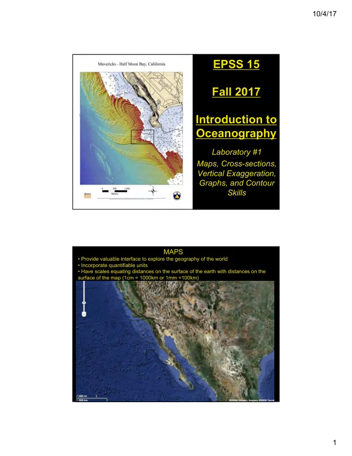
MAPS

• Provide valuable interface to explore the geography of the world
• Incorporate quantifiable units
• Have scales equating distances on the surface of the earth with distances on the

surface of the map (1cm = 1000km or 1mm =100km)

10/4/17 2

Maps, continued

• Latitudes are measured

from 0 – 90 degrees north and south of the equator; they mark points of equal angle above and below the equator

• Longitudes are measured

from 0 - 180 degrees east and west of the prime meridian, which runs from the north to south pole through Greenwich, England Parallels of Latitude Meridians of Longitude

Cross-Sections

• Present a side view of the earth
• Depth dimension allows for

description of the interior of the Earth and subsurface of the oceans.

• In this class, we are primarily

interested in cross-sections illustrating vertical profiles generated through our oceans, and what they can tell us about changes in salinity, temperature, etc and the surface shape of the ocean’s floor.

• The next page shows a portion of an

actual cross-section of part of the earth’s crust below the town of Santa Barbara, CA….

10/4/17 3

Scale: __cm = __km

• This was generated using geometric data observed from the surface of the earth between two

points, & shows the predicted subsurface geometry of rocks.

Cross-Sections

Elevation (kilometers)

0 - 1 - 2 - 3 - 0 10 20 30 40

Distance (kilometers)

Map by P. Coney

Scale is 1 inch = 500 feet

• This was generated using geometric data observed from the surface of the

earth between two points, & shows the predicted subsurface geometry of rocks.

Cross-Sections

Elevation (meters)

Fault Geologic formation contact Bedding

Distance (meters)

Northridge Earthquake Davis & Namson, 1994

10/4/17 4

Vertical exaggeration

• Vertical exaggeration helps maximize the utility of cross-

sections, especially across large distances.

• Earth’s surface is relatively smooth; if Earth were an egg,

the crust of can be equated to the thickness of the

• eggshell. As a result, cross sections often use vertical

exaggeration to show near-surface features.

Vertically exaggerated Not vertically exaggerated

Vertical exaggeration calculations

1. Find horizontal and vertical scales scale = 2. Then, V.E. = 3. For example, if vertical scale = 50 cm , and horizontal scale = 50 cm , 10 km 100 km then, V.E. = 50 cm/10 km = 5 = 10 (ten times) 50 cm/100 km 0.5 Distance represented on map Distance represented on earth Vertical scale Horizontal scale

10/4/17 5

Graphs

• Visualize relationship between two

variables (or more); commonly producing trend lines or curves

• Graphs are useful 2-d

representations of data; data points are plotted on vertical and horizontal axes

• Graphs can portray linear and non-

linear trends of data

Graphs, continued

• Values, and inferences from the data plot can be gained via interpolation

and extrapolation

• Interpolation = Estimating a value from within the known data plot
• Extrapolation = Estimating a value from beyond the known data plot (e.g.

by extending the trend of the curve fitting the pre-existing data to predict a value generated in space beyond the available plot)

• Today, you’ll be working with plotted data values in a nonlinear relationship

Interpolation Extrapolation

10/4/17 6

Contours and Bathymetry

• Contours are lines connecting data

points of equal value (on maps and cross-sections)

• Examples include the following:

– Bathymetry (measurement of depths of

• ceans; e.g. maps on your tables)

– Topography (e.g. USGS quadrangles, hiking maps) – Temperature (e.g. weather maps) – Pressure, density, etc.

• Contours provide spatial knowledge of

the earth’s surface and ocean floor’s surface Three RULES:

• 1. Contours never cross one

another; you can’t be at two different elevations or depths at the same time.

• 2. A contour can close upon itself;

e.g. concentric circles describing a mountain pinnacle, undersea mountain, valley, etc.

• 3. “V’s” that point uphill are troughs

and ones that point downhill are ridges

Contours and Bathymetry

10/4/17 7

Contours and Bathymetry cont.

Bathymetric maps