[PPT] - EMRIs, Kicks & Tails from Black Hole Perturbation Theory (using PowerPoint Presentation

SLIDE 1

7/29/15 AEI Golm 1

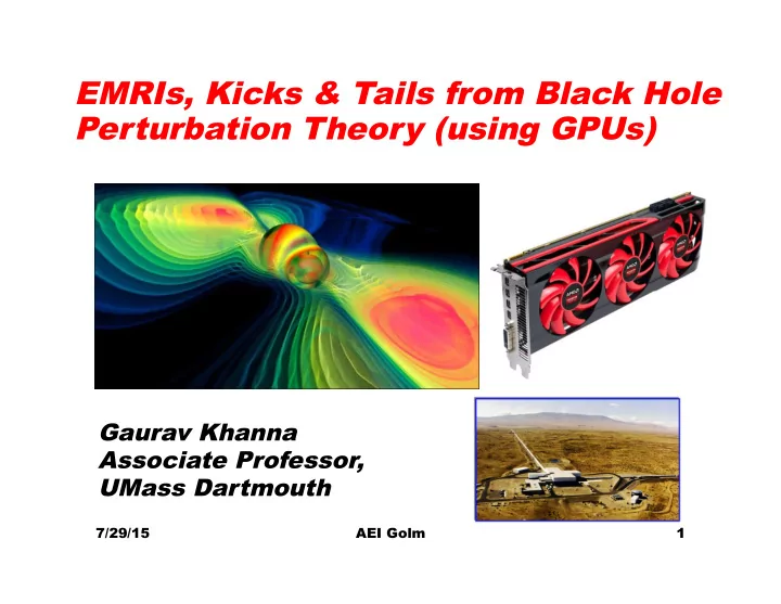
EMRIs, Kicks & Tails from Black Hole Perturbation Theory (using GPUs)

Gaurav Khanna Associate Professor, UMass Dartmouth

SLIDE 2

Collaborators & Support

Alessandra Buonanno, AEI Golm
Lior Burko, Georgia G. College
Scott Hughes, MIT
Richard Price, UTexas / UMassD
P. Sundararajan, MIT, Morgan-Stanley
Andrea Taracchini, AEI Golm
Anil Zenginoglu, UMaryland

Funding: National Science Foundation

7/29/15 2 AEI Golm

SLIDE 3

7/29/15 AEI Golm 3

Talk Outline

EMRIs using BH perturbation theory
Teukolsky equation solver with

particle-source in the time-domain

Waveforms and kicks & anti-kicks
Scalar-field “tails” in BH spacetimes
Kerr BH “tails” controversy
Computing with gaming devices
OpenCL / GPU computing
Summary and Future Outlook

SLIDE 4

Kerr (rotating) black hole perturbation theory

Write Einstein’s GR field equations to linear
rder expanding about a BH solution
Teukolsky equation -- a wave-equation like

PDE that describes how generic fields (scalar, vector, tensor) in the space-time of a Kerr BH behave (propagate/evolve)

In the gravitational field context --

describes the behavior of GWs emitted from Kerr black holes

Relatively simple: linear, hyperbolic, (3+1)D

PDE .. (can be reduced down to (2+1)D)

7/29/15 4 AEI Golm

SLIDE 5

Teukolsky equation

Here -- a: spin of the Kerr black hole M: mass of the Kerr black hole s: spin-weight of the field considered (s is -2 for outgoing GWs)

7/29/15 5 AEI Golm

SLIDE 6

EMRI

7/29/15 6 AEI Golm

EMRI: Extreme-Mass Ratio (binary) Inspiral

SLIDE 7

Point-like compact

bject ..
Source of the GWs (perturbation) in EMRI

is the inspiraling compact object

How to model a point-like compact object

(technically a Dirac-delta function) on a numerical (finite-difference) grid?

Obvious approach would be to take a

narrow Gaussian distribution; do several runs with successively narrower profiles; take some sort of a limit ..

Decent results, but very expensive

7/29/15 7 AEI Golm

SLIDE 8

Discrete Dirac-delta

Alternative approach to representing Dirac-

delta on numerical finite-difference grid

Particularly well suited for numerical

computation (time-domain, finite-difference)

Work done in collaboration with Pranesh

Sundararajan & Scott Hughes (MIT)

Excellent (highly accurate) results
Extremely efficient (by over an order-of-

magnitude)

7/29/15 8 AEI Golm

SLIDE 9

7/29/15 9 AEI Golm

SLIDE 10

Teukolsky Equation

7/29/15 10 AEI Golm

SLIDE 11

7/29/15 11 AEI Golm

SLIDE 12

“source-term” T4

s4 = 1.D0/2.D0 s6 = 1/(r**2+a**2*ctheta**2) s9 = r**2+a**2 s12 = (r+cmplx(0.D0,1.D0)*a*ctheta)/(r**2+a**2*ctheta**2)*sqrt(2.D #0)*(a*stheta*nmu/rp**5*sqrt(2.D0)/dtdT*(E*(a**2+rp**2)-a*lz)*(a*E- #lz)/pie**2/wr*exp(-(r-rp)**2/wr**2/2)/wt*exp(-ctheta**2/wt**2/2)*m #m**2*dphidt**2*exp(cmplx(0.D0,-1.D0)*mm*phip)/16-nmu/rp**5*sqrt(2. #D0)/dtdT*(E*(a**2+rp**2)-a*lz)*(a*E-lz)/pie**2/wr*exp(-(r-rp)**2/w #r**2/2)/wt**3*ctheta*stheta*exp(-ctheta**2/wt**2/2)*mm*dphidt*exp( #cmplx(0.D0,-1.D0)*mm*phip)/16-1/stheta*nmu/rp**5*sqrt(2.D0)/dtdT*( #E*(a**2+rp**2)-a*lz)*(a*E-lz)/pie**2/wr*exp(-(r-rp)**2/wr**2/2)/wt #*exp(-ctheta**2/wt**2/2)*mm**2*dphidt*exp(cmplx(0.D0,-1.D0)*mm*phi #p)/16)/2 s13 = cmplx(0.D0,1.D0/8.D0)*a*(r+cmplx(0.D0,1.D0)*a*ctheta)/(r**2+ #a**2*ctheta**2)**2*(r+cmplx(0.D0,-1.D0)*a*ctheta)*stheta*nmu/rp**5 #/dtdT*(E*(a**2+rp**2)-a*lz)*(a*E-lz)/pie**2/wr*exp(-(r-rp)**2/wr** #2/2)/wt*exp(-ctheta**2/wt**2/2)*mm*dphidt*exp(cmplx(0.D0,-1.D0)*mm #*phip)-(cmplx(0.D0,1.D0/2.D0)*a*(r+cmplx(0.D0,1.D0)*a*ctheta)**2/( #r**2+a**2*ctheta**2)**2*stheta*sqrt(2.D0)-(r+cmplx(0.D0,1.D0)*a*ct #heta)/(r**2+a**2*ctheta**2)/tan(th)*sqrt(2.D0)/4)*nmu/rp**5*sqrt(2 #.D0)/dtdT*(E*(a**2+rp**2)-a*lz)*(a*E-lz)/pie**2/wr*exp(-(r-rp)**2/ #wr**2/2)/wt*exp(-ctheta**2/wt**2/2)*mm*dphidt*exp(cmplx(0.D0,-1.D0 #)*mm*phip)/8 s11 = s12+s13 s12 = s11-1/(r**2+a**2*ctheta**2)*((r**2+a**2)*nmu/rp**4/dtdT*(a*E #-lz)**2/pie**2/wr*exp(-(r-rp)**2/wr**2/2)/wt*exp(-ctheta**2/wt**2/ #2)*mm**2*dphidt**2*exp(cmplx(0.D0,-1.D0)*mm*phip)/8+cmplx(0.D0,1.D #0/8.D0)*(r**2+a**2-2*M*r)*nmu/rp**4/dtdT*(a*E-lz)**2/pie**2/wr**3* #(r-rp)*exp(-(r-rp)**2/wr**2/2)/wt*exp(-ctheta**2/wt**2/2)*mm*dphid #t*exp(cmplx(0.D0,-1.D0)*mm*phip)-a*nmu/rp**4/dtdT*(a*E-lz)**2/pie* #*2/wr*exp(-(r-rp)**2/wr**2/2)/wt*exp(-ctheta**2/wt**2/2)*mm**2*dph #idt*exp(cmplx(0.D0,-1.D0)*mm*phip)/8)/2 s13 = s12+cmplx(0.D0,-1.D0/4.D0)*(-(r+cmplx(0.D0,1.D0)*a*ctheta)** #2/(r**2+a**2*ctheta**2)**3*(r+cmplx(0.D0,-1.D0)*a*ctheta)*(r**2+a* #*2-2*M*r)/2+(r+cmplx(0.D0,1.D0)*a*ctheta)/(r**2+a**2*ctheta**2)**2 #*(r+cmplx(0.D0,-1.D0)*a*ctheta)*(r-M)/2)*nmu/rp**4/dtdT*(a*E-lz)** #2/pie**2/wr*exp(-(r-rp)**2/wr**2/2)/wt*exp(-ctheta**2/wt**2/2)*mm* #dphidt*exp(cmplx(0.D0,-1.D0)*mm*phip)

7/29/15 12 AEI Golm

s15 = -(r+cmplx(0.D0,1.D0)*a*ctheta)/(r**2+a**2*ctheta**2)*sqrt(2. #D0)*(-a*stheta*nmu*(E*(a**2+rp**2)-a*lz)**2/dtdT/rp**6/pie**2/wr*e #xp(-(r-rp)**2/wr**2/2)/wt*exp(-ctheta**2/wt**2/2)*mm*dphidt*exp(cm #plx(0.D0,-1.D0)*mm*phip)/16+nmu*(E*(a**2+rp**2)-a*lz)**2/dtdT/rp** #6/pie**2/wr*exp(-(r-rp)**2/wr**2/2)/wt**3*ctheta*stheta*exp(-cthet #a**2/wt**2/2)*exp(cmplx(0.D0,-1.D0)*mm*phip)/16+1/stheta*nmu*(E*(a #**2+rp**2)-a*lz)**2/dtdT/rp**6/pie**2/wr*exp(-(r-rp)**2/wr**2/2)/w #t*exp(-ctheta**2/wt**2/2)*mm*exp(cmplx(0.D0,-1.D0)*mm*phip)/16)/2 s16 = -(cmplx(0.D0,-1.D0/2.D0)*a*(r+cmplx(0.D0,1.D0)*a*ctheta)/(r* #*2+a**2*ctheta**2)**2*(r+cmplx(0.D0,-1.D0)*a*ctheta)*stheta*sqrt(2 #.D0)+cmplx(0.D0,1.D0)*a*(r+cmplx(0.D0,1.D0)*a*ctheta)**2/(r**2+a** #2*ctheta**2)**2*stheta*sqrt(2.D0))*nmu*(E*(a**2+rp**2)-a*lz)**2/dt #dT/rp**6/pie**2/wr*exp(-(r-rp)**2/wr**2/2)/wt*exp(-ctheta**2/wt**2 #/2)*exp(cmplx(0.D0,-1.D0)*mm*phip)/16 s14 = s15+s16 s10 = s13+s14 s8 = s9*s10 s6 = s7*s8 s8 = cmplx(0.D0,2.D0)*a*(r+cmplx(0.D0,1.D0)*a*ctheta)**2 s10 = 1/((r**2+a**2*ctheta**2)**2)*stheta s12 = sqrt(2.D0) s15 = 1/(r**2+a**2*ctheta**2)*(-(r**2+a**2)*nmu/rp**5*sqrt(2.D0)/d #tdT*(E*(a**2+rp**2)-a*lz)*(a*E-lz)/pie**2/wr*exp(-(r-rp)**2/wr**2/ #2)/wt*exp(-ctheta**2/wt**2/2)*mm*dphidt*exp(cmplx(0.D0,-1.D0)*mm*p #hip)/16+cmplx(0.D0,-1.D0/16.D0)*(r**2+a**2-2*M*r)*nmu/rp**5*sqrt(2 #.D0)/dtdT*(E*(a**2+rp**2)-a*lz)*(a*E-lz)/pie**2/wr**3*(r-rp)*exp(- #(r-rp)**2/wr**2/2)/wt*exp(-ctheta**2/wt**2/2)*exp(cmplx(0.D0,-1.D0 #)*mm*phip)+a*nmu/rp**5*sqrt(2.D0)/dtdT*(E*(a**2+rp**2)-a*lz)*(a*E- #lz)/pie**2/wr*exp(-(r-rp)**2/wr**2/2)/wt*exp(-ctheta**2/wt**2/2)*m #m*exp(cmplx(0.D0,-1.D0)*mm*phip)/16)/2 s16 = cmplx(0.D0,-1.D0/8.D0)*(-(r+cmplx(0.D0,1.D0)*a*ctheta)**2/(r #**2+a**2*ctheta**2)**3*(r+cmplx(0.D0,-1.D0)*a*ctheta)*(r**2+a**2-2 #*M*r)/2+(r+cmplx(0.D0,1.D0)*a*ctheta)/(r**2+a**2*ctheta**2)**2*(r+ #cmplx(0.D0,-1.D0)*a*ctheta)*(r-M)/2)*nmu/rp**5*sqrt(2.D0)/dtdT*(E* #(a**2+rp**2)-a*lz)*(a*E-lz)/pie**2/wr*exp(-(r-rp)**2/wr**2/2)/wt*e #xp(-ctheta**2/wt**2/2)*exp(cmplx(0.D0,-1.D0)*mm*phip) s14 = s15+s16

SLIDE 13

continues ..

7/29/15 13 AEI Golm

s15 = -(r+cmplx(0.D0,1.D0)*a*ctheta)/(r**2+a**2*ctheta**2)*sqrt(2. #D0)*(-a*stheta*nmu*(E*(a**2+rp**2)-a*lz)**2/dtdT/rp**6/pie**2/wr*e #xp(-(r-rp)**2/wr**2/2)/wt*exp(-ctheta**2/wt**2/2)*mm*dphidt*exp(cm #plx(0.D0,-1.D0)*mm*phip)/16+nmu*(E*(a**2+rp**2)-a*lz)**2/dtdT/rp** #6/pie**2/wr*exp(-(r-rp)**2/wr**2/2)/wt**3*ctheta*stheta*exp(-cthet #a**2/wt**2/2)*exp(cmplx(0.D0,-1.D0)*mm*phip)/16+1/stheta*nmu*(E*(a #**2+rp**2)-a*lz)**2/dtdT/rp**6/pie**2/wr*exp(-(r-rp)**2/wr**2/2)/w #t*exp(-ctheta**2/wt**2/2)*mm*exp(cmplx(0.D0,-1.D0)*mm*phip)/16)/2 s16 = -(cmplx(0.D0,-1.D0/2.D0)*a*(r+cmplx(0.D0,1.D0)*a*ctheta)/(r* #*2+a**2*ctheta**2)**2*(r+cmplx(0.D0,-1.D0)*a*ctheta)*stheta*sqrt(2 #.D0)+cmplx(0.D0,1.D0)*a*(r+cmplx(0.D0,1.D0)*a*ctheta)**2/(r**2+a** #2*ctheta**2)**2*stheta*sqrt(2.D0))*nmu*(E*(a**2+rp**2)-a*lz)**2/dt #dT/rp**6/pie**2/wr*exp(-(r-rp)**2/wr**2/2)/wt*exp(-ctheta**2/wt**2 #/2)*exp(cmplx(0.D0,-1.D0)*mm*phip)/16 s14 = s15+s16 s10 = s13+s14 s8 = s9*s10 s6 = s7*s8 s8 = cmplx(0.D0,2.D0)*a*(r+cmplx(0.D0,1.D0)*a*ctheta)**2 s10 = 1/((r**2+a**2*ctheta**2)**2)*stheta s12 = sqrt(2.D0) s15 = 1/(r**2+a**2*ctheta**2)*(-(r**2+a**2)*nmu/rp**5*sqrt(2.D0)/d #tdT*(E*(a**2+rp**2)-a*lz)*(a*E-lz)/pie**2/wr*exp(-(r-rp)**2/wr**2/ #2)/wt*exp(-ctheta**2/wt**2/2)*mm*dphidt*exp(cmplx(0.D0,-1.D0)*mm*p #hip)/16+cmplx(0.D0,-1.D0/16.D0)*(r**2+a**2-2*M*r)*nmu/rp**5*sqrt(2 #.D0)/dtdT*(E*(a**2+rp**2)-a*lz)*(a*E-lz)/pie**2/wr**3*(r-rp)*exp(- #(r-rp)**2/wr**2/2)/wt*exp(-ctheta**2/wt**2/2)*exp(cmplx(0.D0,-1.D0 #)*mm*phip)+a*nmu/rp**5*sqrt(2.D0)/dtdT*(E*(a**2+rp**2)-a*lz)*(a*E- #lz)/pie**2/wr*exp(-(r-rp)**2/wr**2/2)/wt*exp(-ctheta**2/wt**2/2)*m #m*exp(cmplx(0.D0,-1.D0)*mm*phip)/16)/2 s16 = cmplx(0.D0,-1.D0/8.D0)*(-(r+cmplx(0.D0,1.D0)*a*ctheta)**2/(r #**2+a**2*ctheta**2)**3*(r+cmplx(0.D0,-1.D0)*a*ctheta)*(r**2+a**2-2 #*M*r)/2+(r+cmplx(0.D0,1.D0)*a*ctheta)/(r**2+a**2*ctheta**2)**2*(r+ #cmplx(0.D0,-1.D0)*a*ctheta)*(r-M)/2)*nmu/rp**5*sqrt(2.D0)/dtdT*(E* #(a**2+rp**2)-a*lz)*(a*E-lz)/pie**2/wr*exp(-(r-rp)**2/wr**2/2)/wt*e #xp(-ctheta**2/wt**2/2)*exp(cmplx(0.D0,-1.D0)*mm*phip) s14 = s15+s16 s4 = 1.D0/2.D0 s6 = 1/(r**2+a**2*ctheta**2) s9 = r**2+a**2 s12 = (r+cmplx(0.D0,1.D0)*a*ctheta)/(r**2+a**2*ctheta**2)*sqrt(2.D #0)*(a*stheta*nmu/rp**5*sqrt(2.D0)/dtdT*(E*(a**2+rp**2)-a*lz)*(a*E- #lz)/pie**2/wr*exp(-(r-rp)**2/wr**2/2)/wt*exp(-ctheta**2/wt**2/2)*m #m**2*dphidt**2*exp(cmplx(0.D0,-1.D0)*mm*phip)/16-nmu/rp**5*sqrt(2. #D0)/dtdT*(E*(a**2+rp**2)-a*lz)*(a*E-lz)/pie**2/wr*exp(-(r-rp)**2/w #r**2/2)/wt**3*ctheta*stheta*exp(-ctheta**2/wt**2/2)*mm*dphidt*exp( #cmplx(0.D0,-1.D0)*mm*phip)/16-1/stheta*nmu/rp**5*sqrt(2.D0)/dtdT*( #E*(a**2+rp**2)-a*lz)*(a*E-lz)/pie**2/wr*exp(-(r-rp)**2/wr**2/2)/wt #*exp(-ctheta**2/wt**2/2)*mm**2*dphidt*exp(cmplx(0.D0,-1.D0)*mm*phi #p)/16)/2 s13 = cmplx(0.D0,1.D0/8.D0)*a*(r+cmplx(0.D0,1.D0)*a*ctheta)/(r**2+ #a**2*ctheta**2)**2*(r+cmplx(0.D0,-1.D0)*a*ctheta)*stheta*nmu/rp**5 #/dtdT*(E*(a**2+rp**2)-a*lz)*(a*E-lz)/pie**2/wr*exp(-(r-rp)**2/wr** #2/2)/wt*exp(-ctheta**2/wt**2/2)*mm*dphidt*exp(cmplx(0.D0,-1.D0)*mm #*phip)-(cmplx(0.D0,1.D0/2.D0)*a*(r+cmplx(0.D0,1.D0)*a*ctheta)**2/( #r**2+a**2*ctheta**2)**2*stheta*sqrt(2.D0)-(r+cmplx(0.D0,1.D0)*a*ct #heta)/(r**2+a**2*ctheta**2)/tan(th)*sqrt(2.D0)/4)*nmu/rp**5*sqrt(2 #.D0)/dtdT*(E*(a**2+rp**2)-a*lz)*(a*E-lz)/pie**2/wr*exp(-(r-rp)**2/ #wr**2/2)/wt*exp(-ctheta**2/wt**2/2)*mm*dphidt*exp(cmplx(0.D0,-1.D0 #)*mm*phip)/8 s11 = s12+s13 s12 = s11-1/(r**2+a**2*ctheta**2)*((r**2+a**2)*nmu/rp**4/dtdT*(a*E #-lz)**2/pie**2/wr*exp(-(r-rp)**2/wr**2/2)/wt*exp(-ctheta**2/wt**2/ #2)*mm**2*dphidt**2*exp(cmplx(0.D0,-1.D0)*mm*phip)/8+cmplx(0.D0,1.D #0/8.D0)*(r**2+a**2-2*M*r)*nmu/rp**4/dtdT*(a*E-lz)**2/pie**2/wr**3* #(r-rp)*exp(-(r-rp)**2/wr**2/2)/wt*exp(-ctheta**2/wt**2/2)*mm*dphid #t*exp(cmplx(0.D0,-1.D0)*mm*phip)-a*nmu/rp**4/dtdT*(a*E-lz)**2/pie* #*2/wr*exp(-(r-rp)**2/wr**2/2)/wt*exp(-ctheta**2/wt**2/2)*mm**2*dph #idt*exp(cmplx(0.D0,-1.D0)*mm*phip)/8)/2 s13 = s12+cmplx(0.D0,-1.D0/4.D0)*(-(r+cmplx(0.D0,1.D0)*a*ctheta)** #2/(r**2+a**2*ctheta**2)**3*(r+cmplx(0.D0,-1.D0)*a*ctheta)*(r**2+a* #*2-2*M*r)/2+(r+cmplx(0.D0,1.D0)*a*ctheta)/(r**2+a**2*ctheta**2)**2 #*(r+cmplx(0.D0,-1.D0)*a*ctheta)*(r-M)/2)*nmu/rp**4/dtdT*(a*E-lz)** #2/pie**2/wr*exp(-(r-rp)**2/wr**2/2)/wt*exp(-ctheta**2/wt**2/2)*mm* #dphidt*exp(cmplx(0.D0,-1.D0)*mm*phip)

SLIDE 14

… and many more slides!

7/29/15 14 AEI Golm

SLIDE 15

Discrete-delta: Results

For a “static” delta (say, circular-equatorial

particle geodesics) excellent results (Sundararajan, GK, Hughes; Phys. Rev. D 2007)

Improvement (modest) in accuracy over the

Gaussian delta approach (~1% or better energy and angular momentum fluxes)

Dramatic improvement (20x) in performance

(speed) compared with Gaussian delta approach due to need to compute T4 on much fewer grid points!

7/29/15 15 AEI Golm

SLIDE 16

Discrete-delta: Results 2

For a “dynamical” delta (say, eccentric-inclined

particle geodesics) good results (Sundararajan, GK, Hughes, Drasco; Phys. Rev. D 2008)

Movement of the discrete-delta across the grid

points generates numerical noise

Make use of “filtering” on the source-term to

reduce these noise levels

Some loss in accuracy and performance, but

still major improvement over Gaussian-delta approach

7/29/15 16 AEI Golm

SLIDE 17

EMRI waveforms for elliptic-inclined orbit

7/29/15 17 AEI Golm

SLIDE 18

Aside: Frequency- Domain Methods

Teukolsky equation can be solved in frequency-

domain too (its separable -- 3 ODEs!)

Yields extremely accurate results for periodic
rbits
In particular, does very well with computation
f gravitational wave fluxes (energy, angular-

momentum, etc.)

Does relatively very poorly for computation of

waveforms, especially for non-periodic cases (inspiral!)

7/29/15 18 AEI Golm

SLIDE 19

How about a genuine inspiral waveform?

So far we’ve talked about non-decaying

geodesics i.e. without “radiation-reaction”

For an inspiral orbit, we need to include the

effects of radiation reaction (“self-force” will cause decay of the orbit)

This is a difficult problem (CAPRA community)
Partial results are available (mostly for

“dissipative” part of the self-force)

7/29/15 19 AEI Golm

SLIDE 20

How to generate a complete inspiral orbit

There are 3 phases to an orbital decay process
Slow inspiral -- “Slow” decay of the orbit at large

separations (use frequency-domain radiative fluxes to compute the decay in the physical quantities -- E - energy, Lz - ang. mom. & Q - Carter const.)

Plunge geodesic after the ISCO has been crossed
Transition orbit between the above plunge and

inspiral (see work done by Ori & Thorne; Phys.

Rev. D 2000)
For complete details see: Sundararajan; Phys.
Rev. D (2008)

7/29/15 20 AEI Golm

SLIDE 21

EMRI Inspiral Results

Mass-ratio: 0.016 Initial orbit -- p = 10M e = 0.5 θ = 0.5 rad BH spin (a/M) = 0.5 Hybrid approach: time-domain for waveforms & frequency-domain for

rbital decay details

7/29/15 21 AEI Golm

SLIDE 22

Hybrid approach: time-domain for waveforms & frequency-domain for

rbital decay details

7/29/15 22 AEI Golm

SLIDE 23

Other enhancements

Hyperboloidal compactification of

the computational domain

Zenginoglu, GK; Phys. Rev. X

(2011)

Adds a hyperboloidal layer to the
uter domain smoothly
Null infinity on the computational

grid (~50M); solves “outer boundary problem” beautifully; allows for ultra high grid resolutions (~M/500!)

GPU-cluster parallelism (later)

7/29/15 23 AEI Golm

SLIDE 24

a/M = 0.9 r_0 = 5M ~300,000 cycles! (24 hrs, 150 GPUs)

7/29/15 AEI Golm 24

0.01% accuracy!

SLIDE 25

Recoil velocity or “kick”

GWs also carry away linear-momentum flux

from the system

This results in the system experiencing “kick”
r “recoil”
Kicks have been the subject of several NR

papers (may provide a mechanism for the ejection of such binaries from a galaxy)

Our EMRI approach allows us to compute these

recoil velocities too: Sundararajan, GK, Hughes; Phys. Rev. D (2010)

7/29/15 25 AEI Golm

SLIDE 26

7/29/15 AEI Golm 26

Kick Results

Blu a/M= -0.9 Mag a/M= -0.6 Cyn a/M= -0.3 Blk a/M= 0.0 Red a/M= 0.3 Grn a/M= 0.6 Ylw a/M= 0.9 “anti-kick”

SLIDE 27

7/29/15 AEI Golm 27

Why an “anti-kick” ?

Some subtle interaction/

cancellation with the plunge phase GWs?

Uncovered a “simple”

explanation with Richard Price

Nothing subtle going on;

simply due to “slowly” evolving envelope & the high frequency

scillations

SLIDE 28

7/29/15 AEI Golm 28

Trajectory Dominance

The origin of the behavior can

be traced back to the spin- dependence of the plunging trajectories

Prograde case is a slow,

smooth decay – right conditions for “anti-kick”

Retrograde case has abrupt

change in motion resulting in little or no kick cancellation

Price, GK, Hughes; Phys. Rev.

D (2011, 2013)

SLIDE 29

7/29/15 AEI Golm 29

Trajectory Dominance: QNR

Led to the question: perhaps the

trajectory is indeed the dominant feature throughout (to understand the physics)?

BH spacetime is not important for waves;

BH only provides the QNR frequencies

Can we understand plunge and ringdown

waveform in detail using trajectory dominance idea?

Key question: What feature of the

trajectory relates to the QNR amplitude?

SLIDE 30

7/29/15 AEI Golm 30

Trajectory Dominance: QNR 2

Work with Price & Nampalliwar (in progress)
Main insight: the velocity of the particle at

the light-ring determines QNR signal Toss objects into hole on different “cubic” trajectories (but fix velocity at light-ring)

SLIDE 31

7/29/15 AEI Golm 31

Trajectory Dominance: QNR Kerr space-time

Why does that happen? What is special

about the light ring? Is this useful?

There may be an explanation in the context
f behavior of “characteristics” near light

ring (they are almost trapped there ..)

What about Kerr BH? No unique light ring!
Our early tests suggest that only the inner-

most ring (prograde, equatorial) seems to play a role for QNR ..

The next phase of this research ..

SLIDE 32

7/29/15 AEI Golm 32

EOB & Teukolsky Code

Work with AT, AB, Hughes and others ..
Use EOB model to supply inspiral +

plunge trajectories and do Teukolsky evolutions for waveforms

Analyze waveforms, extract important

features and improve EOB model (especially for spin-dependent behavior)

Uncovered a number of interesting

features (time-lag between peaks, QNR mode mixing in retrograde cases)

Phys. Rev. D (2014, 2013, 2012)

SLIDE 33

7/29/15 AEI Golm 33

Kerr BH “Tails”

Late-time decay of

fields in BH space- time is a power-law ~ 1/tn

Richard Price (1972):

Schwarzschild BH the power law index n = 2L+3 (L is the multi pole moment of the field here)

SLIDE 34

7/29/15 AEI Golm 34

“Tails” Controversy

Late-time decay of fields in Kerr space-

time is a power-law ~ 1/tn

Confusion in literature about index n;

various formulae proposed (Hod, Burko) (see for example Burko, GK; CQG 2009) Involve complex analytic approximations and other intuitive arguments (involving mode-mixing and the expectation that Price’s Law should still apply to each multipole mode).

SLIDE 35

7/29/15 AEI Golm 35

Accurate Simulations

Most common numerically studied case:

L=4, m=0 (spin-weight zero; source-free Teukolsky equation is being evolved here!)

Hod’s prediction was n = 5; while the

“common sense” prediction would be n = 3

Now established by several independent

numerical simulations (spectral collocation method Tiglio et al; CQG 2008), higher-

rder finite-difference (Burko, GK; CQG

2009) etc.) that the correct answer is indeed n = 5 (!) i.e. not “common sense” ..

Computations require very high accuracy

and also high precision numerics! Very challenging to attempt ..

SLIDE 36

7/29/15 AEI Golm 36

Sample Results

Study other (higher)

multi-pole modes

Require dramatic

reduction in truncation and round-off errors

Use quadruple and
ctal precision

numerics!

See quality and wide

range of results in preprint: Spilhaus, GK; arXiv:1312.5210 arXiv:1312.5210

SLIDE 37

7/29/15 AEI Golm 37

Splitting?

Why is the “common sense” expectation wrong?
Add more confusion: Racz & Toth; CQG (2011)

noted that near field tails (for some modes) are different than in the far field (!) We were able to show that this “splitting” is intermediate behavior; asymptotically the tail behavior is identical everywhere Zenginoglu, GK, Burko;

Gen. Rel. Grav. (2014)

n

SLIDE 38

7/29/15 AEI Golm 38

Ongoing Work

Why is the “common sense”

expectation wrong?

It has entirely to do with mode

coupling in Kerr space-time

Modes may get excited via

different channels and these may result in different power law rates!

The slowest decay rate

channel dominates in the end,

f course (details matter!)
We have now a “simple”

modified Price law for Kerr

Burko, GK; Phys. Rev. D (2014)

SLIDE 39

7/29/15 AEI Golm 39

NY Times Dec 2014

SLIDE 40

7/29/15 AEI Golm 40

SLIDE 41

7/29/15 AEI Golm 41

Accelerators -- GPUs

There are now “many-core” compute

architectures that have continued to rapidly increase in performance and are designed to do so in the future: Graphics Processing Units (GPUs)

Significantly more power efficient
Much higher performance –

parallelization / vectorization ops

Considered the future of

supercomputing for many years

SLIDE 42

7/29/15 AEI Golm 42

Some Metrics

2nd top (and 20 petaflop/s) system in the

top500.org list is GPU based

9 / 10 top systems in the Green500.org list

are totally GPU based

GPU based systems have an extremely

high power and cost efficiency

Our interest as researchers is simply to get
ur codes to run as fast as possible!

SLIDE 43

7/29/15 AEI Golm 43

Performance Metrics

McKennon, Forrester, GK; XSEDE12 (2012)

(16-core 2.2 GHz Intel Xeon CPU baseline)

Name Name Archit hitect ectur ure e No No. . of

f Cor
res

es Speed peed up up Intel Xeon E5 - 2600

CPU 16 1x

Nvidia Fermi M2050

GPU 500 6x

AMD Radeon Fury X

GPU 4000 18x

SLIDE 44

7/29/15 AEI Golm 44

Coding with OpenCL

OpenCL is a new industry standard (similar to

OpenGL) led by Apple and adopted by all major processor vendors (IBM, Nvidia, AMD/ATI, Intel)

Based on data-parallel model and queues
OpenCL code runs UNCHANGED on CPUs,

GPUs, FPGAs and will do so on future hardware

Tremendous savings on development efforts!
EMRI Teukolsky OpenCL code is the current

version in use for research productivity

SLIDE 45

7/29/15 AEI Golm 45

Summary & Future

BH perturbation theory continues to be

very rich both for mathematical and physical inquiry

Continues to be of potentially great

value to GW astronomy & astrophysics

Even in the present era of full NR, the

computational efficiency and simplicity

f the approach is likely to continue to

yield important and interesting results

Lots of interesting problems to tackle!

SLIDE 46

7/29/15 AEI Golm 46