
SLIDE 1
¡Electron ¡beam ¡proper.es ¡and ¡FEL ¡– ¡Lecture ¡I ¡
Massimo.Ferrario@LNF.INFN.IT ¡
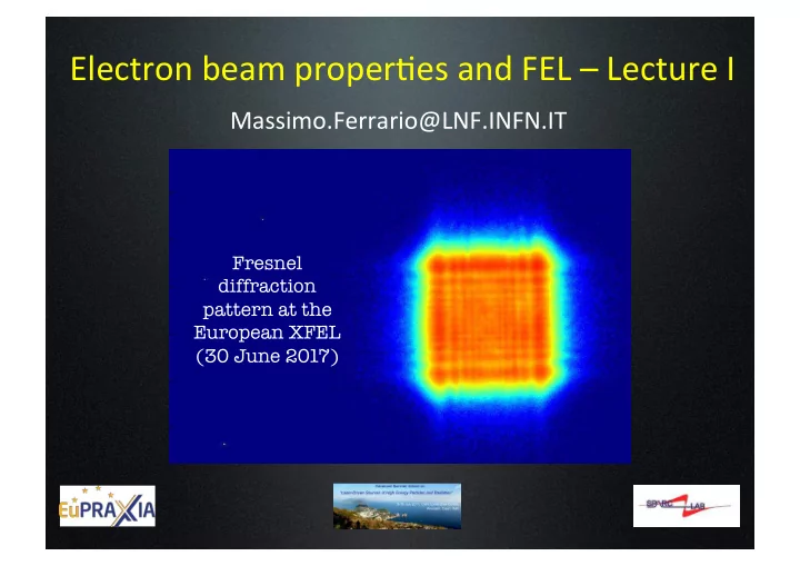
Fresnel diffraction pattern at the European XFEL (30 June 2017)
Electron beam proper.es and FEL Lecture I - - PowerPoint PPT Presentation
Electron beam proper.es and FEL Lecture I Massimo.Ferrario@LNF.INFN.IT Fresnel diffraction pattern at the European XFEL (30 June 2017) LCLS at SLAC 1.5-15 X-FEL based on last 1-km of existing SLAC
Fresnel diffraction pattern at the European XFEL (30 June 2017)
LCLS FLASH XFEL SwissFel FERMI SACLA PAL SDUV
I. Bending magnets in HEP rings
λrad ≈ λu 2γ 2 1 + K 2 2 + γ 2ϑ 2 & ' ( ) * +
SPARX 12.4 1.24 0.124 λ (nm)
http://lcls.slac.stanford.edu/AnimationViewLCLS.aspx
Transverse electron motion in an Undulator:
β// = β 2 − β⊥
2 =
1− 1 γ 2 − β⊥
2 ≈ 1 − 1
2 1 γ 2 + β⊥
2
' ( ) * + ,
β
// = 1−
1 2γ 2 1+ K 2 2 % & ' ( ) *
θ = 1 γ The ¡electron ¡trajectory ¡ is ¡inside ¡ ¡the ¡radia.on ¡ cone ¡if: ¡
The ¡electron ¡trajectory ¡is ¡determined ¡ by ¡ the ¡ undulator ¡ field ¡ and ¡ the ¡ electron ¡energy ¡
β
// = 1 −
1 2γ 2 1 + K 2 2 % & ' ( ) *
! x = K γ cos kuz
( )
λu
' = λu
γ //
'
'
Counter propagating pseudo-radiation Thompson back-scattered radiation in the mirror moving frame
λrad ≈ λu 2γ 2 1+ K 2 2 + γ 2ϑ 2 & ' ( ) * +
Tunability & Red Shift
Doppler effect in the laboratory frame
λrad = γ $ λ
rad 1− β cosϑ
( ) ≈ λu 1− β
// cosϑ
β
// = 1 −
1 2γ 2 1 + K 2 2 % & ' ( ) *
cosϑ ≈ 1 − ϑ 2 2
λrad ≈ λu 2γ 2 1+ K 2 2 +γ 2ϑ 2 " # $ % & '
x 2 = γ 2ε 2
2 = εn 2
2
Energy spread Beam Emittance Undulator tolerances
P
1 =
e2 6πεoc 3 γ 4 ˙ v
⊥ 2
Peak power of one accelerated charge:
P
T = N e 2e2
6πεoc 3 γ 4 ˙ v
⊥ 2
Coherent Stimulated Radiation Power:
P
T = N e
e2 6πεoc 3 γ 4 ˙ v
⊥ 2
Different electrons radiate indepedently hence the total power depends linearly on the number Ne of electrons per bunch: Incoherent Spontaneous Radiation Power: Bunching on the scale of the wavelength:
Spontaneous Emission ==> Random phases N
Coherent Light ==> Stimulated Emission N2
Radiation Simulator – T. Shintake, @ http://www-xfel.spring8.or.jp/Index.htm
Nu = 5
λrad ∝ λu 2γ 2
Letargy Spontaneous Emission Low Gain Slow Bunching Exponential Growth Stimulated emission High Gain Enhanced Bunching Saturation Absorption No Gain Debunching
Energy exchange occurs only if there is transverse motion Consider“seeding”by an external light source with wavelength λr The light wave is co-propagating with the relativistic electron beam
Newton Lorentz Equations Maxwell Equations
Problem: electrons are slower than light Question: can there be a continuous energy transfer from electron beam to light wave? Answer: We need a Self Consistent Model
(R. Bonifacio, C.Pellegrini, L.Narducci, Opt. Comm., 50, 373 (1984))
The relative slippage of the radiation envelope through the electron beam can be neglected, provided that lb>>Nuλr (Steady State Regime) After one wiggler period the electron sees the radiation with the same phase if the flight time delay is exactly one radiation period:
Δt = te − tph = Trad
Δt = λu cβ// − λu c = λrad c & → & λrad = 1− β
//
β
//
λu
β
// ≈1
& → & & λrad ≈ λu 2γ 2 1+ K 2 2 * + ,
/
γ res ≈ λu 2λrad 1 + K 2 2 % & ' ( ) *
In a resonant and randomly phased electron beam, nearly one half of the electrons absorbs energy and one half loses energy, with no net energy exchange.
dγ dt = − e mec Exβx = − eEoK 2γmec cosψ −cosψ
[ ]
Ex z,t
( ) = Eo cos klz − ωlt +ψo ( )
kl = ωl c = 2π λl
Plane wave with constant amplitude , co-propagating with the electron beam:
Ponderomotive phase: Fast oscillating phase (we can neglect it)
βx = K γ cos kuz
( )
Ponderomotive potential
dψ dt = kl + ku
ku<<kl klc
2 1 γr
2 − 1
γ 2 # $ % & ' ( 1+ K 2 2 # $ % & ' ( dψ dt ≈ 2kucγ −γr γr
βz =1− 1 2γ 2 1+ K 2 2 " # $ % & '
γr ≈ λu 2λrad 1+ K 2 2 " # $ % & '
Electrons with energies above the resonant energy move faster, while energies below will make the electrons fall back
Off-resonance electrons motion
t>0 t=0 Optical potential Ponderomotive Potential t=0 …………………………
If the undulator is sufficiently long the energy modulation becomes a phase modulation: the electrons self-bunch on the scale of a radiation wavelength. The particles bunch around a phase where there is weak coupling with the radiation:
ψr
dψ dt ≈ 2kucγ −γr γr dψ dt > 0 for γ >γr dψ dt < 0 for γ <γr # $ % % & % %
t>0 t=0 Optical potential Ponderomotive Potential t=0 …………………………
b z,t
( ) = 1
N e−iψ j
j= 1 N
= e−iψ j
Spontaneous emission Stimulated emission Bunching Parameter:
The Bunching parameter:
For particles with off resonance energy, the ponderomotive phase is no longer constant
Motion in the potential well: the electron pendulum equations
dψ dt ≈ 2kucγ −γr γr = 2kucη dη dt = 1 γr dγ dt = − eEoK 2γr
2mec cosψ
# $ % % & % %
η = γ − γ r γ r << 1
Two coupled first order differential equations
Combining the two coupled first order differential equations:
dψ dt = 2kucη dη dt = − eEoK 2γ r
2mec
cosψ & ' ( ( ) ( (
d 2ψ dt 2 = − eEoKku γ r
2me
cosψ
d 2ψ dt 2 + Ω 2 cosψ = 0
Ω 2 = eEoKku γ r
2me
ηsep = ± eEK kumec 2γ r
2 cos ψ −ψr
2 & ' ( ) * +
ψ ψ
Separatrix
Letargy Exponential Growth Stimulated emission High Gain Enhanced Bunching Saturation Absorption No Gain Debunching
dψ dt = 2kucη dη dt = − eEoK 2γ r
2mec
cosψ & ' ( ( ) ( (
˜ E
x z,t
( ) = ˜
E
x z
( )ei kl z−ωl t
( ) = Eo z
( )eiϕ
2 ei kl z−ωl t
( )
Test solution
∇⊥
2 + ∂ 2
∂z2 − 1 c2 ∂ 2 ∂t2 $ % & ' ( ) Ex z,t
∂ jx ∂t
2ikl ˜ " E
x z
( ) + ˜ "
" E
x z
( )
( ) = µo
∂jx ∂t
Slowly Varying Envelope Approximation (SVEA):
the amplitude variation within one undulator period is very small
˜ " E
x z
( ) <<
˜ E
x z
( )
λu ⇒ ˜ " " E
x z
( ) <<
˜ " E
x z
( )
λu
d˜ E
x z
( )
dz = − iµo 2kl ∂jx ∂t e−i kl z−ωl t
( )
2ikl ˜ " E
x = µo
1 T ∂ ˜ j
x
∂t
t t +T
e−i kl z−ωl t
( )dt
To be consistent with SVEA we should average also the source term
T ≈ n λl c
˜ E
x z
( )
˜ j
x = e
S vxj
j= 1 N
∑
δ z − z j t
( )
( ) =
e Svz vxj
j= 1 N
∑
δ t − t j z
( )
( )
1 T ˜ j
xe−i kl z−ωl t
( )dt
t t +T
= e SvzT vxj
j= 1 N
δ t − t j z
( )
( )e−i kl z−ωl t
( )dt
t t +T
= e V vxj
j= 1 N
e
−i kl z−ωl t j
( ) where : V = SvzT
= e V Kc γ j cos kuz
( )e
−i kl z−ωl t j
( )
j= 1 N
using vxj = ..... = eKc Vγ r e
−i kl +ku
( )z−ωl t j
( )
j= 1 N
= eKc Vγ r e−iψ j
j= 1 N
using γ j ≈ γ r = eKc Vγ r N e−iψ j = eKc γ r ne e−iψ j where ne = N V
1 T ∂ jx ∂t
t t+T
e
−i klz−ωlt
( )dt = −iωl
T jxe
−i klz−ωlt
( ) dt
t t+T
Integration by parts with: Beam model S: transverse beam area Exercise: verify there are not misprints (~mistakes):
∂ 2 jx ∂t2 ≈ 0
−iψ j
2 ℜe
iψ j
b = 1 N e−iψ j
j= 1 N
= e−iψ j
Three coupled first order differential equations. They describe a collective instability of the system which leads to electron self- bunching and to exponential growth of the radiation until saturation effects set a limit on the conversion of electron kinetic energy into radiation energy. Saturation effects prevent the beam to radiate as N2, limting the radiated power scaling to N4/3, due to a competition between neighbours slices . When propagation effects and slippage are relevant, i.e. when the elctron beam is as short as a slippage length, the emitted radiation leaves the bunch before saturation occurs and the power scaling becomes N2 (Super-radiant or Single Spike regime) Bunching parameter
b z,t = 0
˜ E
x z,t = 0
" # $ % $ ⇒ ˜ E
x z,t
2 ℜe
iψ j
b z,t = 0
˜ E
x z,t = 0
# $ % & % ⇒ ˜ E
x z,t
b z,t = 0
˜ E
x z,t = 0
# $ % & % ⇒ ˜ E
x z,t
The particles within a micro-bunch radiate coherently. The resulting strong radiation field enhances the micro-bunching even further. Result: collective instability, exponential growth of radiation power.
Newton Lorentz Equations Maxwell Equations
Letargy Exponential Growth Saturation Absorption No Gain Debunching
dψ dt = 2kucη dη dt = − eEoK 2γ r
2mec
cosψ & ' ( ( ) ( (
d Ex dz = µo 2 eK γr ne e
−iψ j
dψ j dz = 2kucη j dη j dz = − eK 2mec2γr
2 ℜe
Exe
iψ j
( )
# $ % % % & % % %
dψ j dz = 2kucη j
z=2kuρz
! → !!!!!! dψ j dz = cη j ρ = cη dη j dz = − eK 2mec2γr
2 ℜe
Exe
iψ j
A= eK 4kuρ2mec2γr
2 ℜe
Ex
( )
! → !!!!!! dη j dz = −ℜe Ae
iψ j
d Ex dz = µo 2 eK γr ne e
−iψ j
! → !!!!!!! dA dz = 1 ρ3 µone γr
3mec2
eK 4ku % & ' ( ) *
2
+ ,
/ e
−iψ j
1 2 3 3 3 3 4 3 3 3 3
ρ = 1 γr µone mec2 eK 4ku ! " # $ % &
2
' ( ) ) * + , ,
1/3 ene=I/2πcσ x
2
IA=4πmc/eµo
γr 2I IA K 4ckuσ x ! " # $ % &
2
' ( ) ) * + , ,
1/3
iψ j
−iψ j
A
2 + η = const
η
sat = A
sat 2 = −1 ⇒ η sat = Δγ
ργ ≈1 ⇒ Psat = ρP
beam
SASE FEL at short wavelengths require a very intense, high quality e-beam
ρ = 0.136 1 γ r J 1/ 3Bu
2 / 3λu 4 / 3
ρ π λ 3 4
u G
L =
! ! " # $ $ % & =
G
L z P z P exp 9 ) (
ε = εn γ < λ0 4π
P
sat = ρPbeam ∝ Ne 4 / 3
ρ γ γ < Δ
Δω ω = ρ Nu
SASE
Courtesy L. Giannessi (Perseo in 1D mode http://www.perseo.enea.it)
Radiation Simulator – T. Shintake, @ http://www-xfel.spring8.or.jp/Index.htm
The radiation “slips” over the electrons for a distance Nuλrad
ζ
independent processes
Slippage length ≈
SEEDING
Courtesy L. Giannessi (Perseo in 1D mode http://www.perseo.enea.it)
Collider with Integrated X-ray Laser Facility, DESY-1997-048
2
MIN ∝σδ
energy spread undulator parameter minimum radiation wavelength gain length
Bunch compressors (RF & magnetic) Laser Pulse shaping Emittance compensation Cathode emittance
2