einf hrung in visual computing
play

Einfhrung in Visual Computing Unit 12: Local Operations http:// - PowerPoint PPT Presentation

Einfhrung in Visual Computing Unit 12: Local Operations http:// www.caa.tuwien.ac.at/cvl/teaching/sommersemester/evc Content: Neighborhood Introduction to Local Operations Boundary Problem 2D Convolution Linear Image


  1. Einführung in Visual Computing Unit 12: Local Operations http:// www.caa.tuwien.ac.at/cvl/teaching/sommersemester/evc  Content:  Neighborhood  Introduction to Local Operations  Boundary Problem  2D Convolution  Linear Image Filters  
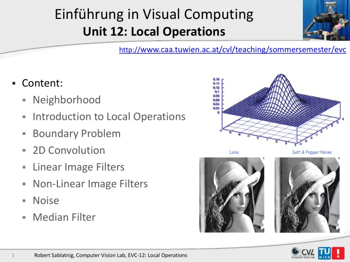
Non-Linear Image Filters  Noise  Median Filter 1 Robert Sablatnig, Computer Vision Lab, EVC-12: Local Operations

  2. Types of Operations  The operations that can be applied to digital images to transform an input image a[m,n] into an output image b[m,n]  Point : the output value at a specific coordinate is dependent only on the input value at that same coordinate.  Local : the output value at a specific coordinate is dependent on the input values in the neighborhood of that same coordinate  Global : the output value at a specific coordinate is dependent on all the values in the input image 2 Robert Sablatnig, Computer Vision Lab, EVC-12: Local Operations

  3. Types of Neighborhoods  Neighborhood operations play a key role in digital image processing  Neighborhoods are basically of two types  4-connected  8-connected  Two types of sampling schemes are  Rectangular sampling - In most cases, images are sampled by laying a rectangular grid over an image  Hexagonal sampling - An alternative sampling scheme 3 Robert Sablatnig, Computer Vision Lab, EVC-12: Local Operations

  4. Types of Neighborhoods (a) (b) Types of neighborhood (a) 4 connected (b) 8 connected 4 Robert Sablatnig, Computer Vision Lab, EVC-12: Local Operations

  5. Local Operations 5

  6. Local-Operations  Point Operators alter image pixel-wise I‘(u,v) = T(I(u,v)). A pixel in the result image depends only on one single pixel in the original image.  Local Operators consider the neighborhood of the pixel too. The locality N of a P(u,v) is given by the surrounding pixels of P(u,v)  The neighborhood is usually square-shaped  Local Operations are very important in image processing. (Usually applied before image analyzing algorithms) 6 Robert Sablatnig, Computer Vision Lab, EVC-12: Local Operations

  7. Local-Operators The Gray level of the resulting pixel is dependent on several pixel in the original image:  An operator window is placed around an actual pixel  Computation of the resulting pixel by combination of gray levels of the actual pixel and its neighbors and saving it at the position of the actual pixel at its position in the result image  Computation of the complete image (by displacement of the operator window by one pixel) Operator window Actual pixel Operator window 7 Robert Sablatnig, Computer Vision Lab, EVC-12: Local Operations

  8. Neighbourhood Operations  For each pixel in the origin image, the outcome is written on the same location at the target image. Origin Target Origin x (x, y) Neighbourhood y Image f (x, y) 8 Robert Sablatnig, Computer Vision Lab, EVC-12: Local Operations

  9. Simple Neighbourhood Operations  Simple neighbourhood operations example:  Min: Set the pixel value to the minimum in the neighbourhood  Max: Set the pixel value to the maximum in the neighbourhood 9 Robert Sablatnig, Computer Vision Lab, EVC-12: Local Operations

  10. The Spatial Filtering Process Origin x a b c j k l * d e f m n o g h i p q r Original Image Filter ( w ) Simple 3*3 Pixels e 3*3 Filter Neighbourhood e processed = n *e + j *a + k *b + l *c + m *d + o *f + p *g + q *h + r *i y Image f (x, y) The above is repeated for every pixel in the original image to generate the filtered image 10 Robert Sablatnig, Computer Vision Lab, EVC-12: Local Operations

  11. Linear 2-D Filter 11 Robert Sablatnig, Computer Vision Lab, EVC-12: Local Operations

  12. Spatial Filtering: Equation Form a b ∑∑ = + + g ( x , y ) w ( s , t ) f ( x s , y t ) = − = − s a t b Filtering can be given in equation form as shown above Notations are based on the image shown to the left 12 Robert Sablatnig, Computer Vision Lab, EVC-12: Local Operations

  13. Example 2D Filter 13 Robert Sablatnig, Computer Vision Lab, EVC-12: Local Operations

  14. Smoothing Spatial Filtering One of the simplest spatial filtering operations we can perform is a smoothing operation  Simply average all of the pixels in a neighbourhood around a central value  Especially useful 1 / 9 1 / 9 1 / 9 in removing noise Simple from images 1 / 9 1 / 9 1 / 9 averaging  Also useful for filter highlighting gross 1 / 9 1 / 9 1 / 9 detail 14 Robert Sablatnig, Computer Vision Lab, EVC-12: Local Operations

  15. Smoothing Spatial Filtering Origin x 1 / 9 1 / 9 1 / 9 104 100 108 * 99 106 98 1 / 9 1 / 9 1 / 9 1 / 9 1 / 9 1 / 9 95 90 85 Original Image Filter 1 / 9 1 / 9 1 / 9 104 100 108 Simple 3*3 3*3 Smoothing Pixels 1 / 9 1 / 9 1 / 9 106 99 98 Neighbourhood Filter 1 / 9 1 / 9 1 / 9 95 90 85 e = 1 / 9 *106 + 1 / 9 *104 + 1 / 9 *100 + 1 / 9 *108 + 1 / 9 *99 + 1 / 9 *98 + 1 / 9 *95 + 1 / 9 *90 + 1 / 9 *85 y Image f (x, y) = 98.3333 The above is repeated for every pixel in the original image to generate the smoothed image 15 Robert Sablatnig, Computer Vision Lab, EVC-12: Local Operations

  16. Definition of a Local Operator  The convolution window is moved over the entire image. 16 Robert Sablatnig, Computer Vision Lab, EVC-12: Local Operations

  17. Image Smoothing Example  The image at the top left is an original image of size 500*500 pixels  The subsequent images show the image after filtering with an averaging filter of increasing sizes 3, 5, 9, 15 and 35  Notice how detail begins to disappear 17 Robert Sablatnig, Computer Vision Lab, EVC-12: Local Operations

  18. Image Smoothing Example 18 Robert Sablatnig, Computer Vision Lab, EVC-12: Local Operations

  19. Image Smoothing Example 19 Robert Sablatnig, Computer Vision Lab, EVC-12: Local Operations

  20. Image Smoothing Example 20 Robert Sablatnig, Computer Vision Lab, EVC-12: Local Operations

  21. Image Smoothing Example 21 Robert Sablatnig, Computer Vision Lab, EVC-12: Local Operations

  22. Image Smoothing Example 22 Robert Sablatnig, Computer Vision Lab, EVC-12: Local Operations

  23. Image Smoothing Example 23 Robert Sablatnig, Computer Vision Lab, EVC-12: Local Operations

  24. Weighted Smoothing Filters  More effective smoothing filters can be generated by allowing different pixels in the neighbourhood different weights in the averaging function  Pixels closer to the 1 / 16 2 / 16 1 / 16 central pixel are more Weighted important averaging 2 / 16 4 / 16 2 / 16  Often referred to as a filter weighted averaging 1 / 16 2 / 16 1 / 16 24 Robert Sablatnig, Computer Vision Lab, EVC-12: Local Operations

  25. Another Smoothing Example By smoothing the original image we get rid of lots of the finer detail which leaves only the gross features for thresholding Original Image Smoothed Image Thresholded Image * Image taken from Hubble Space Telescope 25 Robert Sablatnig, Computer Vision Lab, EVC-12: Local Operations

  26. Photoshop: Other Filters - Custom Filter 26 Robert Sablatnig, Computer Vision Lab, EVC-12: Local Operations

  27. Boundary Problem

  28. Strange Things Happen At The Edges! At the edges of an image we are missing pixels to form a neighbourhood Origin x e e e e e e e y Image f (x, y) 28 Robert Sablatnig, Computer Vision Lab, EVC-12: Local Operations

  29. Strange Things Happen At The Edges! (cont…)  There are a few approaches to dealing with missing edge pixels:  Omit missing pixels: Only works with some filters, Can add extra code and slow down processing  Pad the image: Typically with either all white or all black pixels  Replicate border pixels  Truncate the image 29 Robert Sablatnig, Computer Vision Lab, EVC-12: Local Operations

  30. Boundary Problem  Problem: Border pixels cannot be reached!  Possible solution:  Result image shrinks -2 Pixel in width and height. However this solution is usually not feasible. The image size has to remain constant throughout the entire processing. 30 Robert Sablatnig, Computer Vision Lab, EVC-12: Local Operations

  31. Boundary Problem  Another solution:  Border-Pixel are filled with an intensity value.  Being completely ignorant we could use black. In this case the image remains constant. However a very ugly black border remains. 31 Robert Sablatnig, Computer Vision Lab, EVC-12: Local Operations

  32. Boundary Problem  A somewhat better solution:  Border-Pixel are not processed. They are left untouched with their „old“intensity value. When large sized kernels are used boundary might get visible. 32 Robert Sablatnig, Computer Vision Lab, EVC-12: Local Operations

  33. Convolution

  34. Linear Filter  Output signal at each point = weighted average of local region of input signal  Depends on input signal, pattern of weights  “Filter” H(i,j) = function of weights for linear combination  Basic operation = move filter to some position u, add up i • j times H 1 1 ∑ ∑ ← + + ⋅ I ' ( u , v ) I ( u i , v j ) H ( i , j )  In general: = − = − j 1 i 1 34 Robert Sablatnig, Computer Vision Lab, EVC-12: Local Operations

  35. Convolution f(x) g(x) ∞ ∫ ⋅ = − f ( x ) g ( x ) f ( t ) g ( x t ) dt − ∞ 35 Robert Sablatnig, Computer Vision Lab, EVC-12: Local Operations

Download Presentation
Download Policy: The content available on the website is offered to you 'AS IS' for your personal information and use only. It cannot be commercialized, licensed, or distributed on other websites without prior consent from the author. To download a presentation, simply click this link. If you encounter any difficulties during the download process, it's possible that the publisher has removed the file from their server.

Recommend


More recommend