Einfhrung in Visual Computing Clipping Werner Purgathofer - - PDF document

1

Einführung in Visual Computing

Werner Purgathofer

Institut für Computergraphik und Algorithmen

• 6. Vorlesungseinheit “Computergraphik”

Clipping

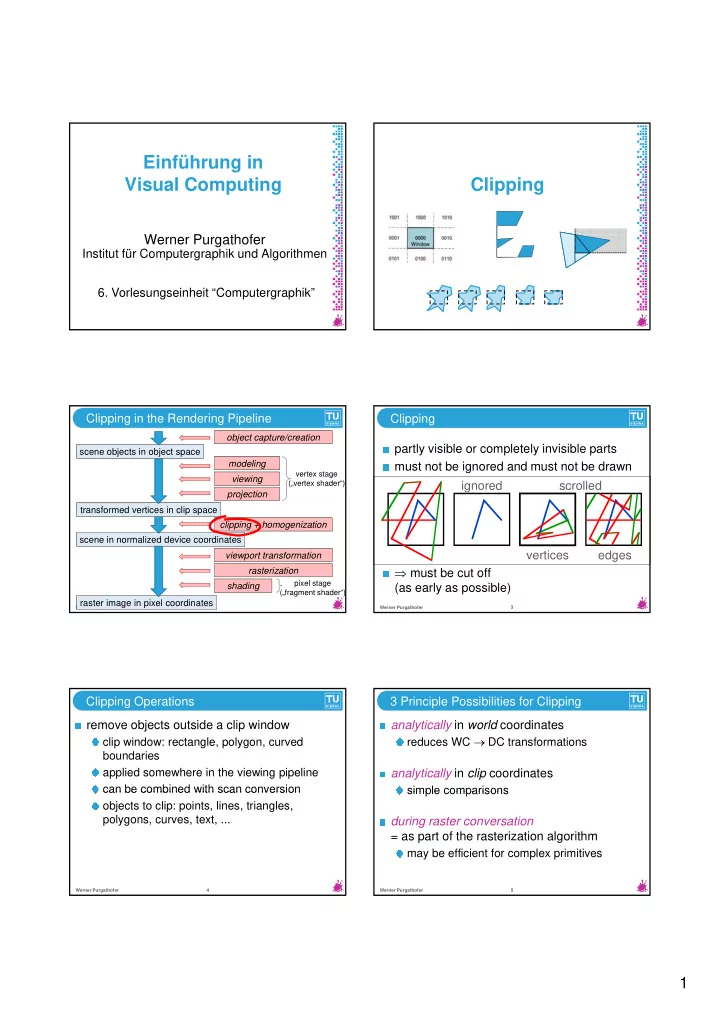
Clipping in the Rendering Pipeline

scene objects in object space

• bject capture/creation

modeling viewing projection

vertex stage („vertex shader“)

transformed vertices in clip space

Werner Purgathofer 2

scene in normalized device coordinates raster image in pixel coordinates clipping + homogenization rasterization viewport transformation shading

pixel stage („fragment shader“)

transformed vertices in clip space

partly visible or completely invisible parts must not be ignored and must not be drawn ignored scrolled Clipping

Werner Purgathofer 3

 must be cut off (as early as possible) vertices edges remove objects outside a clip window

clip window: rectangle, polygon, curved boundaries applied somewhere in the viewing pipeline can be combined with scan conversion

Clipping Operations

Werner Purgathofer 4

can be combined with scan conversion

• bjects to clip: points, lines, triangles,

polygons, curves, text, ...

analytically in world coordinates

reduces WC DC transformations

analytically in clip coordinates

simple comparisons

3 Principle Possibilities for Clipping

Werner Purgathofer 5

simple comparisons

during raster conversation = as part of the rasterization algorithm

may be efficient for complex primitives

2

Line Clipping (1)

P1 P6 P8 P10 P9 P4 P3 P2 P1 P6 P2 P´8

Werner Purgathofer 6

[line clipping against a rectangular clip window]

before clipping after clipping

6

P7 P5 P3

6

P´5 P´7

goals

eliminate simple cases fast avoid intersection calculations

for endpoints (x y ) (x y ) Line Clipping (2)

Werner Purgathofer 7

for endpoints (x0,y0), (xend,yend) intersect parametric representation x = x0 + u(xend  x0) y = y0 + u(yend  y0) with window borders: intersection  0 u  1 assignment of region codes to line endpoints

bit1: left bit2: right bit3: below

Cohen-Sutherland Line Clipping

Werner Purgathofer 8

bit3: below bit4: above

binary region codes assigned to line endpoints according to relative position with respect to the clipping rectangle “or” of codes of both points = 0000  line entirely visible “and” of codes of both Cohen-Sutherland Line Clipping

Werner Purgathofer 9

points  0000  line entirely invisible all others intersect!

[lines extending from one coordinate region to another may pass through

Cohen-Sutherland Line Clipping

Werner Purgathofer 10

may pass through the clip window, or they may intersect clipping boundaries without entering the window]

remaining lines

intersection test with bounding lines of clipping window left, right, bottom, top discard an outside part

Cohen-Sutherland Line Clipping

Werner Purgathofer 11

discard an outside part repeat intersection test up to four times vertical: y = y0 + m(xwmin – x0), y = y0 + m(xwmax – x0) horiz.: x = x0 + (ywmin – y0)/m, x = x0 + (ywmax – y0)/m

3

passes through clipping window intersects boundaries Cohen-Sutherland Line Clipping

Werner Purgathofer 12

without entering clipping window

vertical: y = y0 + m(xwmin – x0), y = y0 + m(xwmax – x0) horiz.: x = x0 + (ywmin – y0)/m, x = x0 + (ywmax – y0)/m

modification of line clipping goal: one or more closed areas Polygon Clipping

Werner Purgathofer 13

[display of a correctly clipped polygon] [display of a polygon processed by a line- clipping algorithm]

Sutherland-Hodgman Polygon Clipping processing polygon boundary as a whole against each window edge

• utput: list of vertices

Werner Purgathofer 14

clipping a polygon against successive window boundaries

• riginal

polygon clip left clip right clip bottom clip top four possible edge cases Sutherland-Hodgman Polygon Clipping

V V V2 V1 V1 V2 V’1

Werner Purgathofer 15

successive processing of pairs of polygon vertices against the left window boundary

• ut  in
• utput: V’1, V2

in  in V2 in  out V’1

• ut  out

no output

V1 V2 V’1 V1 V2

V2:= 1st vertex

for 1 edge:

V1:=V2 V2:=next vertex V2 result list V2 visible?

no yes

Sutherland-Hodgman

Werner Purgathofer 16

V1 visible?

yes

V1 visible?

no

V’1 = clip edge  V1V2 result list

yes no

[clipping a polygon against the left boundary of a window, starting with vertex 1.

Sutherland-Hodgman Polygon Clipping

Werner Purgathofer 17

starting with vertex 1. Primed numbers are used to label the points in the output vertex list for this window boundary]

4

Polygon Clip: Combination of 4 Passes the polygon is clipped against each of the 4 borders separately, that would produce 3 intermediate results. by calling the 4 tests recursively

Werner Purgathofer 18

by calling the 4 tests recursively, (or by using a clipping pipeline) every result point is immediately processed

• n, so that only one result list is produced

2’ 1’ 2

pipeline of boundary clippers to avoid intermediate 1st clip: left Sutherland-Hodgman Clipping Example

Werner Purgathofer 19

2” 3’ 3 1 1’

vertex lists

[Processing the polygon vertices through a boundary-clipping

• pipeline. After all vertices are processed through the pipeline,

the vertex list for the clipped polygon is {1’, 2, 2’, 2”} ]

2nd clip: bottom extraneous lines for concave polygons:

split into separate parts or final check of output vertex list

Sutherland-Hodgman Polygon Clipping

Werner Purgathofer 20

[clipping the concave polygon with the Sutherland- Hodgeman clipper produces three connected areas]

• ften b-reps are “triangle soups”

clipping a triangle  triangle(s) 4 possible cases:

inside t id

Clipping of Triangles

(inside)

Werner Purgathofer 21

• utside

triangle quadrilateral  2 triangles

corner cases need no extra handling! Clipping of Triangles

Werner Purgathofer 22

From Object Space to Screen Space

modeling transformation camera transformation

Werner Purgathofer 23

• bject space

world space camera space clip space screen space

projection transformation viewport transformation

5

clipping against x = ± 1, y = ± 1, z = ± 1 (x,y,z) inside?  only compare one value! Clipping in Clip-Space

Werner Purgathofer 24

is done before homogenization: x = ± h, y = ± h, z = ± h clips points that are behind the camera! reduces homogenization divisions

Antialiasing

Antialiasing in the Rendering Pipeline

scene objects in object space

• bject capture/creation

modeling viewing projection

vertex stage („vertex shader“)

transformed vertices in clip space

Werner Purgathofer 26

scene in normalized device coordinates raster image in pixel coordinates clipping + homogenization rasterization viewport transformation shading

pixel stage („fragment shader“)

transformed vertices in clip space

what is aliasing? ['eiliæsiη] what is the reason for aliasing? Aliasing and Antialiasing

Werner Purgathofer / Computergraphik 1 27

what can we do against it? errors that are caused by the discretization What is Aliasing?

Werner Purgathofer / Computergraphik 1 28

too bad resolution too few colors too few images / sec geometric errors numeric errors

• f analog data to digital data

Aliasing: Staircase Effect

Werner Purgathofer / Computergraphik 1 29

6

Various Aliasing Effects

Werner Purgathofer / Computergraphik 1 30

Aliasing from too few Colors

Werner Purgathofer / Computergraphik 1 31

artificial color borders can appear jumping images "worming“ t Aliasing in Animations

Werner Purgathofer / Computergraphik 1 32

backwards rotating wheels

• 1. improve the devices

higher resolution more color levels faster image sequence

expensive

• r

incompatible Solutions against Aliasing?

Werner Purgathofer / Computergraphik 1 33

• 2. improve the images = antialiasing

postprocessing prefiltering !

software a signal can only be reconstructed without information loss if the sampling frequency is at least twice the highest frequency of the signal Shannon Sampling Theorem

Werner Purgathofer / Computergraphik 1 34

this border frequency is called "Nyquist Limit"

Nyquist

• riginal signal

reconstructed signal Shannon Sampling Theorem

Werner Purgathofer / Computergraphik 1 35

Nyquist sampling interval

sampling rate  

7

a signal can only be reconstructed without information loss if the sampling frequency is at least twice the highest frequency of the signal Antialiasing: Nyquist Sampling Frequency

Werner Purgathofer / Computergraphik 1 36

max cycle

/ 1 x with 2 f x x

cycle s

    

i.e. sampling interval  one-half cycle interval

max

2 f fs 

Nyquist sampling frequency: supersampling straight-line segments subpixel weighting masks area sampling straight-line segments filtering techniques Antialiasing Strategies

Werner Purgathofer / Computergraphik 1 37

compensating for line-intensity differences antialiasing area boundaries

(adjusting boundary pixel positions) adjusting boundary pixel intensity

0 0 0 1 1 0 2 2 2 2 3 1 0 0 0 0 4 4 1 6 6 8 8 8 5 0

Antialiasing: Supersampling Lines

Werner Purgathofer / Computergraphik 1 38

3 1 0 8 5 0

3 = max. intensity ... 0 = min. intensity 9 = max. intensity ... 0 = min. intensity mathematical line line of finite width Antialiasing

Werner Purgathofer / Computergraphik 1 39

more weight for center subpixels must be divided by sum of weights subpixel grids can Antialiasing: Pixel Weighting Masks

Werner Purgathofer / Computergraphik 1 40

relative weights for a grid of 3x3 subpixels subpixel grids can also include some neighboring pixels calculate the pixel coverage exactly can be done with incremental schemes

0% 0% 0% 0% 43% 43% 15% 15% 71% 71% 84% 84% 90% 90% 52% 52% 3% 3%

Antialiasing: Area Sampling Lines

Werner Purgathofer / Computergraphik 1 41

90% 90% 52% 52% 3% 3%

8

continuous overlapping weighting functions to calculate the antialiased values with integrals Antialiasing: Filtering Techniques

Werner Purgathofer / Computergraphik 1 42

box filter cone filter Gaussian filter unequal line lengths displayed with the same number of pixels in each line/row have Antialiasing: Intensity Differences

Werner Purgathofer / Computergraphik 1 43

line/row have different intensities proper antialiasing compensates for that! Antialiasing Area Boundaries

Werner Purgathofer / Computergraphik 1 44

alternative 1: supersampling Antialiasing Area Boundaries (1)

Werner Purgathofer / Computergraphik 1 45

adjusting pixel intensities along an area boundary alternative 2: like midpoint line algorithm p´ = y  ymid = [m(xk + 1) + b]  (yk + 0.5) p´<0  y closer to yk p´>0  y closer to yk+1 Antialiasing Area Boundaries (2)

Werner Purgathofer / Computergraphik 1 46

p = p´+(1m) : p<1m  closer to yk p>1m  closer to yk+1 ( and p  [0,1] ) y ymid p = p´+(1m)= [m(xk + 1) + b]  (yk + 0.5) + (1  m) = mxk + b  yk + 0.5 = = mxk + b  (yk  0.5) yk+ 0.5 p for next pixel = overlap area for current pixel p´ Antialiasing Area Boundaries (3)

Werner Purgathofer / Computergraphik 1 47

xk xk+1 yk m for current pixel p 1-m p p´

9

Antialiasing Area Boundaries (4)

Werner Purgathofer / Computergraphik 1 48

Antialiasing Examples

Werner Purgathofer / Computergraphik 1 49