= y < ymax y > ymin ymax interior X max X min ymin - - PowerPoint PPT Presentation

Why do clipping?

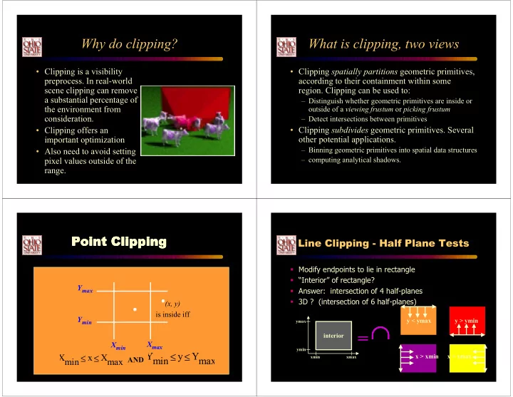
• Clipping is a visibility
• preprocess. In real-world

scene clipping can remove a substantial percentage of the environment from consideration.

• Clipping offers an

important optimization

• Also need to avoid setting

pixel values outside of the range.

What is clipping, two views

• Clipping spatially partitions geometric primitives,

according to their containment within some

• region. Clipping can be used to:

– Distinguish whether geometric primitives are inside or

• utside of a viewing frustum or picking frustum

– Detect intersections between primitives

• Clipping subdivides geometric primitives. Several
• ther potential applications.

– Binning geometric primitives into spatial data structures – computing analytical shadows. Xmin Xmax Ymin Ymax

Point Clipping Point Clipping Point Clipping Point Clipping

(x, y) is inside iff

Xmin x Xmax ≤ ≤

AND Ymin

y Ymax ≤ ≤

y < ymax y > ymin x > xmin x < xmax

=∩

∩ ∩ ∩

interior

xmin xmax ymin ymax

Line Clipping - Half Plane Tests

Modify endpoints to lie in rectangle “Interior” of rectangle? Answer: intersection of 4 half-planes 3D ? (intersection of 6 half-planes)

Line Clipping

Is end-point inside a clip region? - half-plane test If outside, calculate intersection between line and the clipping rectangle and make this the new end point

• Both endpoints inside:

trivial accept

• One inside: find

intersection and clip

• Both outside: either clip or

reject (tricky case)

Cohen-Sutherland Algorithm (Outcode clipping)

• Classifies each vertex of a

primitive, by generating an

• utcode. An outcode

identifies the appropriate half space location of each vertex relative to all of the clipping

• planes. Outcodes are usually

stored as bit vectors.

Cohen-Sutherland Algorithm (Outcode clipping)

if (outcode1 == '0000' and outcode2 == ‘0000’) then line segment is inside else if ((outcode1 AND outcode2) == 0000) then line segment potentially crosses clip region else line is entirely outside of clip region endif endif

The Maybe cases?

If neither trivial accept nor reject: Pick an outside endpoint (with nonzero

• utcode)

Pick an edge that is crossed (nonzero bit of

• utcode)

Find line's intersection with that edge Replace outside endpoint with intersection point Repeat until trivial accept or reject

The Maybe case The Maybe Case The Maybe Case Difficulty

• This clipping will handle most cases.

However, there is one case in general that cannot be handled this way.

– Parts of a primitive lie both in front of and behind the viewpoint. This complication is caused by our projection stage. – It has the nasty habit of mapping objects in behind the viewpoint to positions in front of it.

One Plane At a Time Clipping

• (a.k.a. Sutherland-Hodgeman Clipping)
• The Sutherland-Hodgeman triangle clipping

algorithm uses a divide-and-conquer strategy.

• Clip a triangle against a single plane. Each of the

clipping planes are applied in succession to every triangle.

• There is minimal storage requirements for this

algorithm, and it is well suited for pipelining.

• It is often used in hardware implementations.
• Clip a polygon (input: vertex list) against a single

clip edges

• Output the vertex list(s) for the resulting clipped

polygon(s)

• Clip against all four planes

– Generalizes to 3D (6 planes) – Generalizes to clip against any convex polygon/polyhedron

• Used in viewing transforms

Sutherland-Hodgman Polygon Clipping Algorithm Sutherland-Hodgman Polygon Clipping Algorithm

SHclippedge(var: ilist, olist: list; ilen, olen, edge : integer) s = ilist[ilen];

• len = 0;

for i = 1 to ilen do d := ilist[i]; if (inside(d, edge) then if (inside(s, edge) then

• - case 1 just add d

addlist(d, olist);

• len := olen + 1;

else

• - case 4 add new intersection pt. and d

n := intersect(s, d, edge); addlist(n, olist); addlist(d, olist);

• len = olen + 2;

else if (inside(s, edge) then

• - case 2 add new intersection pt.

n := intersect(s, d, edge); addlist(n, olist); olen ++; s = d; end_for;

Sutherland-Hodgman

Clip input polygon ilist to the edge, edge, and ouput the new polygon.

Sutherland-Hodgman

SHclip(var: ilist, olist: list; ilen, olen : integer) {

SHclippedge(ilist, tmplist1, ilen, tlen1, RIGHT); SHclippedge(tmplist1, tmplist2, tlen1, tlen2, BOTTOM); SHclippedge(tmplist2, tmplist1, tlen2, tlen1, LEFT); SHclippedge(tmplist1, olist, tlen1, olen, TOP);

}

Pictorial Example Sutherland-Hodgman

• Advantages:

– Elegant (few special cases) – Robust (handles boundary and edge conditions well) – Well suited to hardware – Canonical clipping makes fixed-point implementations manageable

• Disadvantages:

– Only works for convex clipping volumes – Often generates more than the minimum number of triangles needed – Requires a divide per edge

Interpolating Parameters

3D Clipping (Planes)

x y z

image plane near far

4D Polygon Clip

Use Sutherland Hodgman algorithm Use arrays for input and output lists There are six planes of course !

• OpenGL uses -1<=x<=1, -1<=y<=1, -1<=z<=1
• We use: -1<=x<=1, -1<=y<=1, -1<=z <=0
• Must clip in homogeneous coordinates:
• w>0: -w<=x<=w, -w<=y<=w, -w<=z<=0
• w<0: -w>=x>=w, -w>=y>=w, -w>=z>=0
• Consider each case separately
• What issues arise ?

4D Clipping

4D Clipping

• Point A is inside, Point B is outside. Clip edge AB

x = Ax + t(Bx – Ax) y = Ay + t(By – Ay) z = Az + t(Bz – Az) w = Aw + t(Bw – Aw)

• Clip boundary: x/w = 1 i.e. (x–w=0);

w-x = Aw – Ax + t(Bw – Aw – Bx + Ax) = 0 Solve for t.

Why Homogeneous Clipping

• Efficiency/Uniformity: A single clip procedure is

typically provided in hardware, optimized for canonical view volume.

• The perspective projection canonical view volume

can be transformed into a parallel-projection view volume, so the same clipping procedure can be used.

• But for this, clipping must be done in homogenous

coordinates (and not in 3D). Some transformations can result in negative W : 3D clipping would not work.

Difficulty (revisit)

• Clipping will handle most cases. However,

there is one case in general that cannot be handled this way.

– Parts of a primitive lie both in front of and behind the viewpoint. This complication is caused by our projection stage. – It has the nasty habit of mapping objects in behind the viewpoint to positions in front of it.

• Solution: clip in homogeneous coordinate

P1 and P2 map to same physical point ! Solution: Clip against both regions Negate points with negative W

4D Clipping Issues

P2=[-1,-2,-3,-4] W=1 P1=[1,2,3,4] W=-X W=X P1 W=1 Inf

• Inf

4D Clipping Issues

Line straddles both regions After projection one gets two line segments How to do this? Only before the perspective division

Additional Clipping Planes

• At least 6 more clipping planes available
• Good for cross-sections
• Modelview matrix moves clipping plane
• clipped
• glEnable( GL_CLIP_PLANEi )
• glClipPlane( GL_CLIP_PLANEi, GLdouble*

coeff )

< + + + D Cz By Ax

Reversing Coordinate Projection

• Screen space back to world space
• glGetIntegerv( GL_VIEWPORT, GLint viewport[4] )
• glGetDoublev( GL_MODELVIEW_MATRIX, GLdouble mvmatrix[16]

)

• glGetDoublev( GL_PROJECTION_MATRIX,

GLdouble projmatrix[16] )

• gluUnProject( GLdouble winx, winy, winz,

mvmatrix[16], projmatrix[16], GLint viewport[4], GLdouble *objx, *objy, *objz )

• gluProject goes from world to screen space

Shaders

• Local illumination quite complex

– Reflectance models – Procedural texture – Solid texture – Bump maps – Displacement maps – Environment maps

• Need ability to collect into a single

shading description called a shader

• Shaders also describe

– lights, e.g. spotlights – atmosphere, e.g. fog

Shading v. Modeling

• Shaders generate more than color

– Displacement maps can move geometry – Opacity maps can create holes in geometry

• Frequency of features

– Low frequency modeling operations – High frequency shading operations

Shade Trees

• Cook, SIGGRAPH 84
• Hierarchical
• rganization of shading
• Breaks a shading

expression into simple components

• Visual programming
• Modular
• Drag-n-drop shading

components

* +

copper color

*

ka Ca

*

ks specular normal viewer roughness

Texture v. Bump Mapping

• Texture

mapping simulates detail with a color that varies across a surface

• Bump mapping

simulates detail with a surface normal that varies across a surface

+ * *

tex(s,t) N L ks kd H

+ * *

tex(s,t) bump() L ks kd H N B

⋅ ⋅ ⋅ ⋅

Problems with Shade Trees

• Shaders can get very complex
• Sometimes need higher-level constructs

than simple expression trees

– Variables – Iteration

• Need to compile a program instead of

evaluate an expression

Renderman Shading Language

• Hanrahan & Lawson, SIGGRAPH 90
• High level little language
• Special purpose variables useful for shading

– P – surface position – N – surface normal

• Special purpose functions useful for shading

– smoothstep(x0,x1,a) – smoothly interpolates from x0 to x1 as a varies from 0 to 1 – specular(N,V,m) – computes specular reflection given normal N, view direction V and roughness m.

Types

• Colors

– Multiplication is componentwise – e.g. Cd*(La + Ld) + Cs*Ls + Ct*Lt

• Points

– Built in dot (L.N) and cross (N^L) products – Transform to other coordinate systems: “raster,” “screen,” “camera,” “world,” and “object”

• Variables

– Uniform – independent of position – Varying – changes across surface

Lighting

• Constructs

– illuminate() – point source with cone spread – solar() – directional source

• Variables

– L – direction of light (independent) – Cl – color of light (dependent)

• Types

– ambient – non-directional (but can vary with position) – point – equal in all directions – spot – focused around a given direction – shadowed – modulated by texture/shadow map – distant –directional source – environment map – distant source modulated by texture

Local Illumination

• Construct

– illuminance()

• Variables

– L – incoming light direction – Cl – incoming light color – C – output color

• Example (hair diffuse)

color C = 0; illuminance(P,N,Pi/2) { L = normalize(L); C += Kd * Cd * Cl * length(L^T); }

Texture Functions

• texture() returns float/color based on texture

coordinates

• bump() returns normal perturbation based
• n texture coordinates
• environment() returns float/color based on a

direction passed to it

• shadow() returns a float indicating the

percentage a point’s position is shadowed

Renderman Example

Surface dent(float Ks=.4, Kd=.5, Ka=.1, roughness=.25, dent=.4) { float turbulence; point Nf, V; float I, freq; /* Transform to solid texture coordinate system */ V = transform(“shader”,P); /* Sum 6 octaves of noise to form turbulence */ turbulence = 0; freq = 1.0; for (i = 0; i < 6; i += 1) { turbulence += 1/freq + abs(0.5*noise(4*freq*V)); freq *= 2; } /* sharpen turbulence */ turbulence *= turbulence * turbulence; turbulence *= dent; /* Displace surface and compute normal */ P -= turbulence * normalize(N); Nf = faceforward(normalize(calculatenormal(P)),I); V = normalize(-I); /* Perform shading calculations */ Oi = 1 – smoothstep(0.03,0.05,turbulence); Ci = Oi*Cs*(Ka*ambient() + Ks*specular(Nf,V,roughness)); }

Try It Yourself

• Photorealistic Renderman

– Based on REYES polygon renderer – Uses shadow maps

• Blue Moon Rendering Tools

– Free – Uses ray tracer – No displacement maps – http://www.exluna.com/products/bmrt/

Deferred Shading

• Makes procedural shading more efficient
• Why apply shader to entire surface if only small

portion is actually visible

• Separate rendering into two passes

– Pass 1: Render geometry using Z-buffer

• But rather than storing color in frame buffer
• Store shading parameters instead

– Pass 2: Shade frame buffer

• Apply shading procedure to frame buffer
• Replaces shading parameters with color
• Problem: Fat framebuffer

OpenGL Architecture

Display List Polynomial Evaluator Per Vertex Operations & Primitive Assembly Rasterization Per Fragment Operations Frame Buffer Texture Memory

CPU

Pixel Operations

Per-Fragment Operations

Display List Polynomial Evaluator Per Vertex Operations & Primitive Assembly Rasterization Per Fragment Operations Frame Buffer Texture Memory

CPU

Pixel Operations

Getting to the Framebuffer

Blending Blending Depth Test Depth Test Dithering Dithering Logical Operations Logical Operations Scissor Test Scissor Test Stencil Test Stencil Test Alpha Test Alpha Test Fragment Framebuffer

Scissor Box

• Additional Clipping Test
• glScissor( x, y, w, h )

– any fragments outside of box are clipped – useful for updating a small section of a viewport

• affects glClear() operations

Alpha Test

• Reject pixels based on their alpha value
• glAlphaFunc( func, value )
• glEnable( GL_ALPHA_TEST )

– use alpha as a mask in textures

Stencil Buffer

• Used to control drawing based on values in

the stencil buffer

– Fragments that fail the stencil test are not drawn – Example: create a mask in stencil buffer and draw only objects not in mask area

Stencil Testing

• Now broadly supports by both major APIs

– OpenGL – DirectX 6

• RIVA TNT and other consumer cards now

supporting full 8-bit stencil

• Opportunity to achieve new cool effects and

improve scene quality

What is Stenciling?

• Per-pixel test, similar to depth buffering.
• Tests against value from stencil buffer;

rejects fragment if stencil test fails.

• Distinct stencil operations performed when

– Stencil test fails – Depth test fails – Depth test passes

• Provides fine grain control of pixel update

OpenGL API

• glEnable/glDisable(GL_STENCIL_TEST);
• glStencilFunc(function, reference, mask);
• glStencilOp(stencil_fail,

depth_fail, depth_pass);

• glStencilMask(mask);
• glClear(… | GL_STENCIL_BUFFER_BIT);

Controlling Stencil Buffer

• glStencilFunc( func, ref, mask )

– compare value in buffer with ref using func – only applied for bits in mask which are 1 – func is one of standard comparison functions

• glStencilOp( fail, zfail, zpass )

– Allows changes in stencil buffer based on passing or failing stencil and depth tests: GL_KEEP, GL_INCR

Request a Stencil Buffer

• If using stencil, request sufficient bits of stencil
• Implementations may support from zero to 32 bits
• f stencil
• 8, 4, or 1 bit are common possibilities
• Easy for GLUT programs:

glutInitDisplayMode(GLUT_DOUBLE | GLUT_RGB | GLUT_DEPTH | GLUT_STENCIL); glutCreateWindow(“stencil example”);

Stencil Test

• Compares reference value to pixel’s stencil buffer

value

• Same comparison functions as depth test:

– NEVER, ALWAYS – LESS, LEQUAL – GREATER, GEQUAL – EQUAL, NOTEQUAL

• Bit mask controls comparison

((ref & mask) op (svalue & mask))

Stencil Operations

• Stencil side effects of

– Stencil test fails – Depth test fails – Depth test passes

• Possible operations

– Increment, Decrement (saturates) – Increment, Decrement (wrap, DX6 option) – Keep, Replace – Zero, Invert

• Way stencil buffer values are controlled

Stencil Write Mask

• Bit mask for controlling write back of

stencil value to the stencil buffer

• Applies to the clear too!
• Stencil compare & write masks allow

stencil values to be treated as sub-fields

Very Complex Clip Window

Digital Dissolve

Creating a Mask

• gluInitDisplayMode(…|GLUT_STENCIL|…);
• glEnable( GL_STENCIL_TEST );
• glClearStencil( 0x0 );
• glStencilFunc( GL_ALWAYS, 0x1, 0x1 );
• glStencilOp( GL_REPLACE, GL_REPLACE,

GL_REPLACE );

• draw mask

Using Stencil Mask

• Draw objects where stencil = 1
• glStencilFunc( GL_EQUAL, 0x1, 0x1 )
• Draw objects where stencil != 1
• glStencilFunc( GL_NOTEQUAL, 0x1, 0x1

);

• glStencilOp( GL_KEEP, GL_KEEP, GL_KEEP

);

Performance

• With today’s 32-bit graphics accelerator

modes, 24-bit depth and 8-bit stencil packed in same memory word

• RIVA TNT is an example
• Performance implication:

if using depth testing, stenciling is at NO PENALTY

Repeating that!

• On card like RIVA TNT2 in 32-bit mode

if using depth testing, stenciling has NO PENALTY

• Do not treat stencil as “expensive” --

in fact, treat stencil as “free” when already depth testing

Pseudo Global Lighting Effects

• OpenGL’s light model is a “local” model

– Light source parameters – Material parameters – Nothing else enters the equation

• Global illumination is fancy word for real-world

light interactions

– Shadows, reflections, refractions, radiosity, etc.

• Pseudo global lighting is about clever hacks

Planar Reflections

Dinosaur is reflected by the planar floor. Easy hack, draw dino twice, second time has glScalef(1,-1,1) to reflect through the floor

Compare Two Versions

Good. Bad. Notice right image’s reflection falls off the floor!

Stencil Maintains the Floor

Clear stencil to zero. Draw floor polygon with stencil set to one. Only draw reflection where stencil is one.

Recursive Planar Mirrors

Basic idea of planar reflections can be applied

• recursively. Requires more stencil bits.

The Trick (bird’s eye view)

Next: Planar Shadows

Shadow is projected into the plane of the floor.

Constructing a Shadow Matrix

void shadowMatrix(GLfloat shadowMat[4][4], GLfloat groundplane[4], GLfloat lightpos[4]) { GLfloat dot; /* Find dot product between light position vector and ground plane normal. */ dot = groundplane[X] * lightpos[X] + groundplane[Y] * lightpos[Y] + groundplane[Z] * lightpos[Z] + groundplane[W] * lightpos[W]; shadowMat[0][0] = dot - lightpos[X] * groundplane[X]; shadowMat[1][0] = 0.f - lightpos[X] * groundplane[Y]; shadowMat[2][0] = 0.f - lightpos[X] * groundplane[Z]; shadowMat[3][0] = 0.f - lightpos[X] * groundplane[W]; shadowMat[X][1] = 0.f - lightpos[Y] * groundplane[X]; shadowMat[1][1] = dot - lightpos[Y] * groundplane[Y]; shadowMat[2][1] = 0.f - lightpos[Y] * groundplane[Z]; shadowMat[3][1] = 0.f - lightpos[Y] * groundplane[W]; shadowMat[X][2] = 0.f - lightpos[Z] * groundplane[X]; shadowMat[1][2] = 0.f - lightpos[Z] * groundplane[Y]; shadowMat[2][2] = dot - lightpos[Z] * groundplane[Z]; shadowMat[3][2] = 0.f - lightpos[Z] * groundplane[W]; shadowMat[X][3] = 0.f - lightpos[W] * groundplane[X]; shadowMat[1][3] = 0.f - lightpos[W] * groundplane[Y]; shadowMat[2][3] = 0.f - lightpos[W] * groundplane[Z]; shadowMat[3][3] = dot - lightpos[W] * groundplane[W]; }

How to Render the Shadow

/* Render 50% black shadow color on top of whatever the floor appearance is. */ glEnable(GL_BLEND); glBlendFunc(GL_SRC_ALPHA, GL_ONE_MINUS_SRC_ALPHA); glDisable(GL_LIGHTING); /* Force the 50% black. */ glColor4f(0.0, 0.0, 0.0, 0.5); glPushMatrix(); /* Project the shadow. */ glMultMatrixf((GLfloat *) floorShadow); drawDinosaur(); glPopMatrix();

Note Quite So Easy (1)

Without stencil to avoid double blending

• f the shadow pixels:

Notice darks spots

• n the planar shadow.

Solution: Clear stencil to zero. Draw floor with stencil

• f one. Draw shadow if stencil is one. If shadow’s

stencil test passes, set stencil to two. No double blending.

Note Quite So Easy (2)

There’s still another problem even if using stencil to avoid double blending. depth buffer Z fighting artifacts Shadow fights with depth values from the floor plane. Use polygon offset to raise shadow polygons slightly in Z.

Everything All At Once

Lighting, texturing, planar shadows, and planar reflections all at one time. Stencil & polygon offset eliminate aforementioned artifacts.

Pseudo Global Lighting

• Planar reflections and shadows add more than

simplistic local lighting model

• Still not really global

– Techniques more about hacking common cases based

• n knowledge of geometry

– Not really modeling underlying physics of light

• Techniques are “multipass”

– Geometry is rendered multiple times to improve the rendered visual quality

Bonus Stenciled Halo Effect

Halo does not obscure

• r blend with the

haloed object. Halo is blended with objects behind haloed object.

Clear stencil to zero. Render object, set stencil to one where object is. Scale up object with

• glScalef. Render object again, but not where

stencil is one.

Other Stencil Uses

• Digital dissolve effects
• Handling co-planar geometry such as decals
• Measuring depth complexity
• Constructive Solid Geometry (CSG)

Digital Dissolve

Stencil buffer holds dissolve pattern. Stencil test two scenes against the pattern

Co-planar Geometry

Shows “Z fighting” of co-planar geometry Stencil testing fixes “Z fighting”

Visualizing Depth Complexity

Use stencil to count pixel updates, then color code results.

Dithering

• glEnable( GL_DITHER )
• Dither colors for better looking results

– Used to simulate more available colors

Logical Operations on Pixels

• Combine pixels using bitwise logical operations
• glLogicOp( mode )

– Common modes

• GL_XOR – Rubberband user-interface.
• GL_AND

– Others

• GL_CLEAR, GL_SET , GL_COPY,
• GL_COPY_INVERTED, GL_NOOP, GL_INVERT
• GL_AND, GL_NAND, GL_OR
• GL_NOR, GL_XOR, GL_AND_INVERTED
• GL_AND_REVERSE, GL_EQUIV, GL_OR_REVERSE
• GL_OR_INVERTED

Imaging and Raster Primitives

• Describe OpenGL’s raster primitives:

bitmaps and image rectangles

• Demonstrate how to get OpenGL to read

and render pixel rectangles

CPU CPU DL DL Poly. Poly. Per Vertex Per Vertex Raster Raster Frag Frag FB FB Pixel Pixel Texture Texture

Pixel-based primitives

• Bitmaps

– 2D array of bit masks for pixels

• update pixel color based on current color
• Images

– 2D array of pixel color information

• complete color information for each pixel
• OpenGL doesn’t understand image formats

May 22-26, 2000 Dagstuhl Visualization Frame Buffer Rasterization (including Pixel Zoom) Per Fragment Operations Texture Memory Pixel-Transfer Operations (and Pixel Map) CPU Pixel Storage Modes

glReadPixels(), glCopyPixels() glBitmap(), glDrawPixels() glCopyTex*Image();

Pixel Pipeline

• Programmable pixel storage

and transfer operations

Positioning Image Primitives

• glRasterPos3f( x, y, z )

– raster position transformed like geometry – discarded if raster position is outside of viewport

• may need to fine tune

viewport for desired results

Raster Position

Rendering Bitmaps

• glBitmap( width, height, xorig, yorig,

xmove, ymove, bitmap )

– render bitmap in current color at – advance raster position by after rendering    

( )

yorig y xorig x − −

( )

ymove xmove

width height xorig yorig xmove

Rendering Fonts using Bitmaps

• OpenGL uses bitmaps for font rendering

– each character is stored in a display list containing a bitmap – window system specific routines to access system fonts

• glXUseXFont()
• wglUseFontBitmaps()

Rendering Images

• glDrawPixels( width, height, format,

type, pixels )

– render pixels with lower left of image at current raster position – numerous formats and data types for specifying storage in memory

• best performance by using format and type that

matches hardware

Reading Pixels

• glReadPixels( x, y, width, height, format,

type, pixels )

– read pixels from specified (x,y) position in framebuffer – pixels automatically converted from framebuffer format into requested format and type

• Framebuffer pixel copy
• glCopyPixels( x, y, width, height, type )

Raster Position

glPixelZoom(1.0, -1.0);

Pixel Zoom

• glPixelZoom( x, y )

– expand, shrink or reflect pixels around current raster position – fractional zoom supported

• glPixelZoom( x, y )

– expand, shrink or reflect pixels around current raster position – fractional zoom supported

Storage and Transfer Modes

• Storage modes control accessing memory

– byte alignment in host memory – extracting a subimage

• Transfer modes allow modify pixel values

– scale and bias pixel component values – replace colors using pixel maps

Immediate Mode versus Display Listed Rendering

• Immediate Mode Graphics

– Primitives are sent to pipeline and display right away – No memory of graphical entities

• Display Listed Graphics

– Primitives placed in display lists – Display lists kept on graphics server – Can be redisplayed with different state – Can be shared among OpenGL graphics contexts

Display Lists

CPU CPU DL DL Poly. Poly. Per Vertex Per Vertex Raster Raster Frag Frag FB FB Pixel Pixel Texture Texture

Immediate Mode versus Display Lists

Immediate Mode Display Listed Display List Polynomial Evaluator Per Vertex Operations & Primitive Assembly Rasterization Per Fragment Operations Texture Memory

CPU

Pixel Operations Frame Buffer

Display Lists

• Creating a display list

GLuint id; void init( void ) { id = glGenLists( 1 ); glNewList( id, GL_COMPILE ); /* other OpenGL routines */ glEndList(); }

• Call a created list

void display( void ) { glCallList( id ); }

Display Lists

• Not all OpenGL routines can be stored in display

lists

• State changes persist, even after a display list is

finished

• Display lists can call other display lists
• Display lists are not editable, but you can fake it

– make a list (A) which calls other lists (B, C, and D) – delete and replace B, C, and D, as needed

Display Lists and Hierarchy

• Consider model of a car

– Create display list for chassis – Create display list for wheel

• glNewList( CAR, GL_COMPILE );
• glCallList( CHASSIS );
• glTranslatef( … );
• glCallList( WHEEL );
• glTranslatef( … );
• glCallList( WHEEL );
• …
• glEndList();

Advanced Primitives

• Vertex Arrays
• Vertex Arrays

CPU CPU DL DL Poly. Poly. Per Vertex Per Vertex Raster Raster Frag Frag FB FB Pixel Pixel Texture Texture

Vertex Arrays

• Pass arrays of vertices, colors, etc. to OpenGL in a

large chunk

glVertexPointer( 3, GL_FLOAT, 0, coords ) glColorPointer( 4, GL_FLOAT, 0, colors ) glEnableClientState( GL_VERTEX_ARRAY ) glEnableClientState( GL_COLOR_ARRAY ) glDrawArrays( GL_TRIANGLE_STRIP, 0, numVerts );

• All active arrays are used in rendering
• Pass arrays of vertices, colors, etc. to OpenGL in a

large chunk

glVertexPointer( 3, GL_FLOAT, 0, coords ) glColorPointer( 4, GL_FLOAT, 0, colors ) glEnableClientState( GL_VERTEX_ARRAY ) glEnableClientState( GL_COLOR_ARRAY ) glDrawArrays( GL_TRIANGLE_STRIP, 0, numVerts );

• All active arrays are used in rendering

Color data Vertex data

Why use Display Lists or Vertex Arrays?

• May provide better performance than immediate

mode rendering

– Avoid function call overheads and small packet sends.

• Display lists can be shared between multiple

OpenGL context

– reduce memory usage for multi-context applications

• Vertex arrays may format data for better memory

access

Alpha: the 4th Color Component

• Measure of Opacity

– simulate translucent objects

• glass, water, etc.

– composite images – antialiasing – ignored if blending is not enabled

glEnable( GL_BLEND )

CPU CPU DL DL Poly. Poly. Per Vertex Per Vertex Raster Raster Frag Frag FB FB Pixel Pixel Texture Texture

Blending

• Combine pixels with what’s in already

in the framebuffer

• glBlendFunc( src, dst )

Framebuffer Framebuffer Pixel Pixel ( (dst dst) )

Blending Equation Blending Equation

Fragment Fragment ( (src src) ) Blended Blended Pixel Pixel

p f r

C dst C src C

• +

=

Multi-pass Rendering

• Blending allows results from multiple

drawing passes to be combined together

– enables more complex rendering algorithms

Example of bump-mapping done with a multi-pass OpenGL algorithm