Efficient Spherical Designs with Good Geometric Properties Rob - - PowerPoint PPT Presentation

Efficient Spherical Designs with Good Geometric Properties

Rob Womersley, R.Womersley@unsw.edu.au

School of Mathematics and Statistics, University of New South Wales

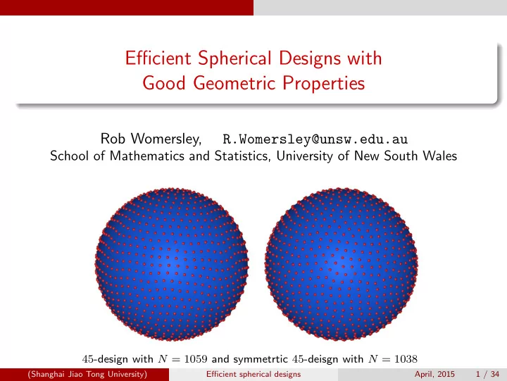
45-design with N = 1059 and symmetrtic 45-deisgn with N = 1038

(Shanghai Jiao Tong University) Efficient spherical designs April, 2015 1 / 34

Outline

1

Spherical designs Spheres and point sets Aims Spherical polynomials Number of points

2

Characterizations Nonlinear equations Variational characterizations Examples Evaluating At,N,ψ(XN) Degrees of freedom for S2 Numerical results

3

Geometric properties Mesh norm Separation Mesh ratio

4

Conclusions

(Shanghai Jiao Tong University) Efficient spherical designs April, 2015 2 / 34

Spherical designs Spheres and point sets

Unit sphere

Unit sphere Sd =

• x ∈ Rd+1 : |x| = 1
• Sets of points XN = {x1, . . . , xN} ⊂ Sd

x · y =

d+1

• i=1

xiyi, |x|2 = x · x

Distance

Euclidean distance: x, y ∈ Sd, |x − y|2 = 2(1 − x · y) Geodesic distance: x, y ∈ Sd, dist (x, y) = arccos(x · y)

Can choose points or given points (scattered data) Want sequences of point sets XN, often as part of integration/approximation problem

(Shanghai Jiao Tong University) Efficient spherical designs April, 2015 3 / 34

Spherical designs Spheres and point sets

Geometric quality of point set

Spherical cap centre z ∈ Sd, radius α C (z; α) =

• x ∈ Sd : dist (x, z) ≤ α
• Separation (twice packing radius):

δXN = min

i=j dist (xi, xj)

Mesh norm (covering radius): hXN = max

x∈Sd

min

j=1,...,N dist (x, xj)

Mesh ratio: ρXN =

2hXN δXN ≥ 1

Desire: ρXN ≤ c

(Shanghai Jiao Tong University) Efficient spherical designs April, 2015 4 / 34

Spherical designs Aims

Aims

Numerical integration (cubature) QN(f) :=

N

• j=1

wjf(xj) ≈ I(f) :=

• Sd f(x)dω(x)

Equal weights wj = |Sd|/N, j = 1, . . . , N (Quasi Monte-Carlo rules) Degree of precision t if exact for all polynomials of degree ≤ t

Spherical t-design is a set XN of N points such that 1 N

N

• j=1

p(xj) = 1 |Sd|

• Sd p(x)dω(x)

∀p ∈ Pt(Sd),

N point, equal weight wj = |Sd|

N

cubature rule, degree of precision t

Efficient: Low number of points N Good geometric properties: Quasi-uniform: Mesh ratio ρX ≤ c

(Shanghai Jiao Tong University) Efficient spherical designs April, 2015 5 / 34

Spherical designs Spherical polynomials

Spherical Polynomials

Space Pt ≡ Pt

• Sd
• f spherical polynomials of degree at most t

Dimension of space of homogeneous harmonic polynomials of degree ℓ Z(d, 0) = 1; Z(d, ℓ) = (2ℓ + d − 1)Γ(ℓ + d − 1) Γ(d)Γ(ℓ + 1) , Orthonormal basis Yℓ,k, ℓ = 0, 1, 2, . . ., k = 1, . . . , Z(d, ℓ) Dimension Pt

• Sd

is D(d, t) = Z(d + 1, t) ≍ td Addition Theorem

Z(d,ℓ)

• k=1

Yℓ,k(x)Yℓ,k(y) = Z(d, ℓ) |Sd| P (d+1)

ℓ

(x · y),

Normalized Gegenbauer polynomial P (d+1)

ℓ

(z) = P( d−2

2 , d−2 2 ) ℓ

(z) P( d−2

2 , d−2 2 ) ℓ

(1)

Jacobi polynomial P (α,β)

ℓ

(z) for z ∈ [−1, 1]

(Shanghai Jiao Tong University) Efficient spherical designs April, 2015 6 / 34

Spherical designs Number of points

Spherical t-designs – Number of points N

Delsarte, Goethals and Seidel (1977)N point t-design on Sd N ≥ N ∗(d, t) :=    2 d+m

d

• if t = 2m + 1,

d+m

d

• +

d+m−1

d

• if t = 2m.

Positive weight cubature, degree of precision t = ⇒ N ≥ dim P⌊t/2⌋(Sd) On S2: N ∗(2, t) = (t + 1)(t + 3)/4 for t odd; (t + 2)2/4 for t even Improved by Yudin (1997) by exponential factor (e/4)d+1 as t → ∞.

Bannai and Damerell (1979, 1980)

Tight spherical t-designs if achieve lower bounds Cannot exist on S2 except for t = 1, 2, 3, 5

Seymour and Zaslavsky (1984) t-designs exist for N sufficiently large Bondarenko, Radchenko and Viazovska (2011, 2013, 2015) On Sd

spherical t-designs exist for N ≥ cd td well-separated spherical t-designs exist for N ≥ c′

d td

(Shanghai Jiao Tong University) Efficient spherical designs April, 2015 7 / 34

Spherical designs Number of points

Existence Results for S2

Bajnok (1991)construction with N = O(t3)

n points z1, . . . , zn, t-design on [−1, 1] Regular m-gon at latitudes zj N = mn point t-design if m ≥ t + 1

Korevaar and Meyers (1993)

N = O(t3)

Both depend on t-designs for interval [−1, 1]

Set of n points zj ∈ [−1, 1]: 2 n

n

• j=1

p(zj) = 1

−1

p(z)dz ∀p ∈ Pt([−1, 1]) Equal weights = ⇒ n = O(t2) points Survey Gautschi (2004)

Tensor product constructions based on 1-D existence result

(Shanghai Jiao Tong University) Efficient spherical designs April, 2015 8 / 34

Spherical designs Number of points

Evidence for S2

Hardin and Sloane (1996)

Summary of known results for S2 Conjecture N = t2 2 (1 + o(1))

N = (t + 1)2 = dim

• Pt(S2)
• Start from extremal (maximum determinant) points

Sloan, W. (2004) Under-determined system of equations Use interval methods to verify a nearby solution

Chen and W. (2006) Chen, Frommer, Lang (2009) An, Chen, Sloan, W. (2010)

(Shanghai Jiao Tong University) Efficient spherical designs April, 2015 9 / 34

Spherical designs Number of points

Number of points, dimension of space

D(d, t) = dimension of space of polynomials of degree ≤ t on Sd DGS lower bound N ∗(d, t) Ratio of leading terms of D(d, t)/N ∗(d, t) = 2d Efficient if N < D(d, t) d N ∗(d, t) N D(d, t) 2

t2 4 + t + O(1)

(t + 1)2 3

t3 24 + 3t2 8 + O(t) t3 3 + O(t2)

4

t4 192 + t3 12 + O(t2) t4 12 + O(t3)

5

t5 1920 + 5t4 384 + O(t3) t5 60 + O(t4)

(Shanghai Jiao Tong University) Efficient spherical designs April, 2015 10 / 34

Spherical designs Number of points

Spherical Harmonic Basis matrix

Spherical Harmonic Basis matrix Y =

• Y0,1eT
• Y
• ∈ RD(d,t)×N

Rows = basis functions, Columns = points e = (1, 1, . . ., 1)T ∈ RN

Consider case N ≤ D(d, t) Gram matrix G = YT Y = Y 2

0,1eeT +

YT Y ∈ RN×N Addition Theorem implies Gii =

t

• ℓ=0

Z(d, ℓ) |Sd| P (d+1)

ℓ

(xi · xi) = D(d, t) |Sd|

Fixed diagonal elements so trace(G) = ND(d,t)

|Sd|

constant

(Shanghai Jiao Tong University) Efficient spherical designs April, 2015 11 / 34

Characterizations Nonlinear equations

Spherical designs – nonlinear equations

Delsarte, Goethals and Seidel (1977) XN = {x1, . . . , xN} ⊂ Sd is a spherical t-design if and only if rℓ,k(XN) :=

N

• j=1

Yℓ,k(xj) = 0 for k = 1, . . . , Z(d, ℓ), ℓ = 1, . . . , t.

Constant (ℓ = 0) polynomial Y0,1 = 1/

• |Sd| not included in (12)

Integral of all spherical harmonics of degree ℓ ≥ 1 is zero Weyl sums: In matrix form r(XN) := Ye = 0

e = (1, . . . , 1)T ∈ RN

• Y ∈ RD(d,t)−1×N, Spherical harmonic basis matrix excluding first row

(Shanghai Jiao Tong University) Efficient spherical designs April, 2015 12 / 34

Characterizations Variational characterizations

Polynomials with positive Legendre coefficients

Polynomial ψt ∈ Pt[−1, 1] with positive coefficients ψt(z) :=

t

• ℓ=1

at,ℓP (τ,τ)

ℓ

(z), at,ℓ > 0 for ℓ = 1, . . . , t.

P (τ,τ)

ℓ

(z) for z ∈ [−1, 1] Jacobi polynomial, parameter τ = d−2

2

1

−1 ψt(z)dz = 0

Variational form At,N,ψ(XN) := 1 N 2

N

• i=1

N

• j=1

ψt(xi · xj)

(Shanghai Jiao Tong University) Efficient spherical designs April, 2015 13 / 34

Characterizations Variational characterizations

Spherical designs – variational characterizations

t ≥ 1, XN = {x1, . . . , xN} ⊂ Sd, Then 0 ≤ At,N,ψ(XN) ≤

t

• ℓ=1

at,ℓ = ψt(1) At,N,ψ := 1 (|Sd|)N

• Sd · · ·
• Sd At,N,ψ(x1, . . . , xN)dω(x1) · · · dω(xN) = ψt(1)

N XN is a spherical design if and only if At,N,ψ(XN) = 0. Weighted sum of squares, strictly positive coefficients At,N,ψ(XN) = |Sd| N 2

t

• ℓ=1

at,ℓ Z(d, ℓ)

Z(d,ℓ)

• k=1

(rℓ,k(XN))2 At,N,ψ(XN) = 0 ⇐ ⇒ XN spherical t-design Global min At,N,ψ(XN) > 0 = ⇒ no spherical t-design with N points

(Shanghai Jiao Tong University) Efficient spherical designs April, 2015 14 / 34

Characterizations Examples

Examples

Grabner and Tichy (1993) ψt(z) = zt + zt−1 − at,0 at,0 =

• 1

t

t odd,

1 t+1

t even. Cohn and Kumar (2007) ψt(z) = (1 + z)t − 2t t + 1. Sloan and W. (2009) ψt(z) = 1 4πP (1,0)

t

(z) − 1 =

t

• ℓ=1

Z(d, ℓ)Pℓ(z)

P (1,0)

t

Jacobi polynomial

(Shanghai Jiao Tong University) Efficient spherical designs April, 2015 15 / 34

Characterizations Evaluating At,N,ψ(XN )

Evaluating At,N,ψ(XN)

Matrix Ψ: Ψij = ψt(xi · xj), i, j = 1, . . . , N Spherical t-design ⇐ ⇒ D(d, t) − 1 equations r := Ye = 0, Diagonal matrix D of weights Ψ = |Sd| YT D Y D = diag

• at,ℓ

Z(d, ℓ), k = 1, . . . , Z(d, ℓ), ℓ = 1, . . . , t

• Any symmetric positive definite D possible

Minimize At,N,ψ(XN) = 1 N 2 eT Ψe = |Sd| N 2 eT YT D Ye = |Sd| N 2 rT Dr

(Shanghai Jiao Tong University) Efficient spherical designs April, 2015 16 / 34

Characterizations Evaluating At,N,ψ(XN )

Evaluating At,N,ψ(XN) using Ψ

N by N matrix Ψij = ψt(xi · xj) Constant diagonal elements ψt(1) = t

ℓ=1 at,ℓ

Matrix Ψ for at,ℓ = Z(d, ℓ) ⇐ ⇒ D = I Advantages: simple, (trivially) parallel Issue: cancelation errors in summing off diagonal elements

(Shanghai Jiao Tong University) Efficient spherical designs April, 2015 17 / 34

Characterizations Degrees of freedom for S2

Degrees of freedom for S2

Spherical parametrization, normalization = ⇒ n = 2N − 3 variables m = dim(Pt) − 1 = (t + 1)2 − 1 equations Threshold n ≥ m = ⇒ N ≥ N(2, t) :=

• (t + 1)2)/2
• + 1
• N less than twice the DGS lower bound N ∗

2N ∗(2, t) − N(2, t) = t, Sum of squares for t = 19, varying N,

• N(2, 19) = 201

100 110 120 130 140 150 160 170 180 190 200 210 10

−30

10

−25

10

−20

10

−15

10

−10

10

−5

10 10

5

Number of points N Residual SSQ rT r for t = 19

(Shanghai Jiao Tong University) Efficient spherical designs April, 2015 18 / 34

Characterizations Degrees of freedom for S2

Symmetric designs

Exploit symmetry to reduce conditions: Sobolev (1962) Symmetric: N even, x ∈ XN ⇐ ⇒ −x ∈ XN Equal weights, ℓ odd = ⇒ Yℓ,k integrated exactly Constraints from even degrees ≤ t, t odd m =

(t−1)/2

• k=1

2(2k) + 1 = (t − 1)(t + 2) 2 N = 2K points = ⇒ 2K − 3 = N − 3 degrees of freedom Degrees of freedom ≥ number of equations = ⇒ N ≥ N(2, t) := 2 t2 + t + 4 4

• Slightly less than

N(2, t) 2N ∗(2, t) − N(2, t) = 3

2t −

3

2

if mod (t, 4) = 1,

1 2

if mod (t, 4) = 3.

(Shanghai Jiao Tong University) Efficient spherical designs April, 2015 19 / 34

Characterizations Degrees of freedom for S2

Degrees of freedom Sd

Sd ⊂ Rd+1: Spherical parametrization = ⇒ d variables N points xj, j = 1, . . . , N = ⇒ Nd variables Orthogonal invariance = ⇒ Qxj so d(d + 1)/2 zero elements Number of variables n = Nd − d(d + 1)/2 Number of equations for t-design m =

t

• ℓ=1

Z(d, ℓ) = Z(d + 1, t) − 1 Number of variables ≥ number of conditions = ⇒ N(d, t) Symmetric point set (both xj, −xj in set) automatically integrates

• dd degree polynomial =

⇒ N(d, t)

(Shanghai Jiao Tong University) Efficient spherical designs April, 2015 20 / 34

Characterizations Degrees of freedom for S2

Number of points, dimension of space

D(d, t) = dimension of space of polynomials of degree ≤ t on Sd DGS lower bound N ∗(d, t)

• N(d, t) ensures n ≥ m

N(d, t) ensures symmetric point set has n ≥ m Ratio of leading terms of D(d, t)/ N(d, t) = d d N ∗(d, t) N(d, t)

• N(d, t)

D(d, t) 2

t2 4 + t + O(1) t2 2 + t 2 + O(1) t2 2 + t + O(1)

(t + 1)2 3

t3 24 + 3t2 8 + O(t) t3 9 + t2 3 + O(t) t3 9 + t2 2 + O(t) t3 3 + O(t2)

4

t4 192 + t3 12 + O(t2) t4 48 + t3 8 + O(t2) t4 48 + t3 6 + O(t2) t4 12 + O(t3)

5

t5 1920 + 5t4 384 + O(t3) t5 300 + t4 30+)(t3) t5 300 + t4 24+)(t3) t5 60 + O(t4)

(Shanghai Jiao Tong University) Efficient spherical designs April, 2015 21 / 34

Characterizations Degrees of freedom for S2

Least squares

Spherical parametrization of variables x ∈ Rn Residuals r : Rn → Rm, m = t

ℓ=1 Z(d, ℓ)

Number of points chosen so n = m or n = m + 1. Sum of squares objective f(x) = r(x)T r(x) = m

i=1[ri(x)]2

Jacobian A(x) ∈ Rm×n Gradient ∇f(x) = 2A(x)r(x) Hessian ∇2f(x) = 2A(x)T A(x) + 2 m

i=1 ri(x)∇2ri(x)

r(x∗) = 0 and A(x∗) rank n = ⇒ strict (isloated) global minimum n > m have some freedom Algorithm: Levenberg-Marquardt (AT A + λI)d = −AT r Issues

Singular Jacobians A(x) Stuck with ∇f(x) = 0 but f(x) > 0, perhaps small Different solutions: depends on starting point, algorithm parameters, ...

(Shanghai Jiao Tong University) Efficient spherical designs April, 2015 22 / 34

Characterizations Numerical results

Spherical designs - numerical results

Use N = N(2, t), = ⇒ t odd, n = m, t even, n = m + 1 Rounding error limits achievable accuracy in At,N Both At,N,ψ(XN), rT r order of rounding error = ⇒ what confidence? t = 180 = ⇒ N(2, t) = 16382, m = 32760, n = 32761

Degree t

20 40 60 80 100 120 140 160 180 10 -32 10 -30 10 -28 10 -26 10 -24 10 -22 10 -20 10 -18

Residual ssq for spherical t-designs

http://web.maths.unsw.edu.au/~rsw/Sphere/EffSphDes/

(Shanghai Jiao Tong University) Efficient spherical designs April, 2015 23 / 34

Characterizations Numerical results

Spherical designs - rate of convergence

Rate of convergence: t = 45, N = 1059, m = 2115, n = 2115

20 40 60 80 100 120 140 160 180 200 220 10

−24

10

−20

10

−16

10

−12

10

−8

10

−4

10 Iterations Sum of squares SSQ for t = 45, N = 1059, m = 2115, n = 2115

(Shanghai Jiao Tong University) Efficient spherical designs April, 2015 24 / 34

Characterizations Numerical results

Spherical designs - Jacobian singular values

Jacobian singular values: t = 45, N = 1059, m = 2115, n = 2115

200 400 600 800 1000 1200 1400 1600 1800 2000 10

−3

10

−2

10

−1

10 10

1

10

2

10

3

Jacobian singular values: t = 45, N = 1059, m = 2115, n = 2115

(Shanghai Jiao Tong University) Efficient spherical designs April, 2015 25 / 34

Characterizations Numerical results

Symmetric spherical designs - numerical results

For t odd, use N = N(2, t)

mod (t, 4) = 3 = ⇒ n = m, mod (t, 4) = 1 = ⇒ n = m + 1

t = 277 = ⇒ N(2, t) = 38506, m = 38502, n = 38503

Degree t

50 100 150 200 250 300 10-32 10-30 10-28 10-26 10-24 10-22 10-20 10-18

Symmetric spherical t-designs, SSQ

http://web.maths.unsw.edu.au/~rsw/Sphere/EffSphDes/

(Shanghai Jiao Tong University) Efficient spherical designs April, 2015 26 / 34

Geometric properties Mesh norm

Mesh norm

Mesh norm (covering radius) hXN = max

x∈S2

min

j=1,...,N dist (x, xj) ≥ ccov

√ N

Yudin (1995) Mesh norm h given by largest zero zt = cos(h) of P (1,0)(z) Reimer (2003) extended to any positive weight cubature rule with degree of precision t

10

1

10

2

10

3

10

4

10

−2

10

−1

10 Number of points N Spherical t−desgins, Mesh norm Mesh norm h(XN) 2.534 N−0.498

(Shanghai Jiao Tong University) Efficient spherical designs April, 2015 27 / 34

Geometric properties Separation

Separation

Separation (twice packing radius) δXN = min

i=j dist (xi, xj) ≤

cpack √ N

Union of two spherical t-designs is a spherical t-design XN ∪ QXN is 2N point spherical t-design with arbitrary separation N < 2N ∗, N < 2N ∗ so cannot occur

If N sufficiently small get separation ?

10

1

10

2

10

3

10

4

10

−2

10

−1

10 Number of points N Spherical t−desgins, Separation Separation δ(XN) 3.078 N−0.502

(Shanghai Jiao Tong University) Efficient spherical designs April, 2015 28 / 34

Geometric properties Mesh ratio

Mesh ratio

Mesh ratio ρXN = 2hXN δXN = Covering radius Packing radius ≥ 1 ρXN bounded = ⇒ XN quasi-uniform Spherical t-designs with N points

Degree t

20 40 60 80 100 120 140 160 180 1 1.1 1.2 1.3 1.4 1.5 1.6 1.7 1.8 1.9 2

Spherical t-designs, Mesh ratio

(Shanghai Jiao Tong University) Efficient spherical designs April, 2015 29 / 34

Geometric properties Mesh ratio

Mesh ratio - Symmetric t-designs

Mesh ratio for symmetric t-designs with N points

Degree t

50 100 150 200 250 300 1 1.1 1.2 1.3 1.4 1.5 1.6 1.7 1.8 1.9 2

Symmetric spherical t-designs, Mesh ratio

Converge to different spherical designs from different starting points If n = m, r∗ = 0 and σn(A∗) > 0 = ⇒ strict global minimizer If n = m + 1 use freedom to reduce mesh ratio

(Shanghai Jiao Tong University) Efficient spherical designs April, 2015 30 / 34

Geometric properties Mesh ratio

Reducing mesh ratio - one degree of freedom

• 0.05
• 0.04
• 0.03
• 0.02
• 0.01

0.01 0.02 0.03 0.04 0.05 ×10-5 0.5 1 1.5 2

Symmetric 53-design: nv = 1431, nc = 1430, tangent to r = 0, SSQ

• 0.05
• 0.04
• 0.03
• 0.02
• 0.01

0.01 0.02 0.03 0.04 0.05 1.7004 1.7006 1.7008 1.701 1.7012 1.7014

Symmetric 53-design: nv = 1431, nc = 1430, tangent to r = 0, RHO (Shanghai Jiao Tong University) Efficient spherical designs April, 2015 31 / 34

Geometric properties Mesh ratio

Reducing mesh ratio - isolated zero

• 0.05
• 0.04
• 0.03
• 0.02
• 0.01

0.01 0.02 0.03 0.04 0.05 ×10-6 1 2 3 4

Symmetric 55-design, nv = 1539, nc = 1539, σ1538 = 1.46e-01, SSQ

• 0.05
• 0.04
• 0.03
• 0.02
• 0.01

0.01 0.02 0.03 0.04 0.05 1.7185 1.719 1.7195 1.72 1.7205

Symmetric 55-design, nv = 1539, nc = 1539, σ1538 = 1.46e-01, RHO (Shanghai Jiao Tong University) Efficient spherical designs April, 2015 32 / 34

Geometric properties Mesh ratio

Starting points

Close to spherical design (low sums of squares) Good mesh ratio Generalized spiral points Equal area points

50 100 150 200 250 300 1000 2000 3000 4000 5000 6000 7000 8000 9000 Symmetric equal areas points: SSQ Degree t 50 100 150 200 250 300 1 1.1 1.2 1.3 1.4 1.5 1.6 1.7 1.8 1.9 2 Symmetric equal areas points: Mesh ratio

(Shanghai Jiao Tong University) Efficient spherical designs April, 2015 33 / 34

Conclusions

Conclusions

Efficient sets of (numerical) t-designs for S2

http://web.maths.unsw.edu.au/~rsw/Sphere/EffSphDes/ Equal weight cubature rule, degree of precision t with

• N = (t2 + 2t)/2 + O(1) points for t = 1, . . . , 180

Symmetric equal weight cubature rule, degree of precision t with N = (t2 + t)/2 + O(1) points for t = 1, . . . , 277 Good geometric properties: mesh norm, separation, mesh ratio < 1.8 Larger N: Use extra degrees of freedom to satisfy other criteria

Issues

Rounding errors in evaluating criteria, speed of extended precision Convergence difficulties with close to singular Jacobians No proof of nearby exact spherical designs when N < (t + 1)2 No proof of existence for all t There exist t-designs with N < N(d, t); special symmetries Calculation by optimization for each t, N Finding points sets with better mesh ratio ad-hoc Point sets XN not nested Higher dimensions d

(Shanghai Jiao Tong University) Efficient spherical designs April, 2015 34 / 34