Efficient Algorithms and Problem Complexity Divide and Conquer - PowerPoint PPT Presentation
Efficient Algorithms and Problem Complexity Divide and Conquer Frank Drewes Department of Computing Science Ume a University Frank Drewes (Ume a University) Efficient Algorithms and Problem Complexity Lecture 2 1 / 14 Outline
Efficient Algorithms and Problem Complexity – Divide and Conquer – Frank Drewes Department of Computing Science Ume˚ a University Frank Drewes (Ume˚ a University) Efficient Algorithms and Problem Complexity Lecture 2 1 / 14
Outline Today’s Menu What is a Divide-and-Conquer Algorithm? 1 Example 1: Mergesort 2 Example 2: Matrix Multiplication 3 Frank Drewes (Ume˚ a University) Efficient Algorithms and Problem Complexity Lecture 2 2 / 14
What is a Divide-and-Conquer Algorithm? Divide et impera (divide and rule) Historically A quote attributed to Julius Caesar describing the political (social, . . . ) strategy to divide those you want to keep under control into competing groups having roughly the same power, so that none of them can become a leader with the power to threaten you. In computer science The problem solving strategy that consists in dividing an input into smaller ones, solving them recursively, and combining the solutions to a solution for the original input. Frank Drewes (Ume˚ a University) Efficient Algorithms and Problem Complexity Lecture 2 3 / 14
What is a Divide-and-Conquer Algorithm? General pattern (1) For a problem instance (input) I is of size n . . . divide I into a smaller instances I 1 , . . . , I a , solve I 1 , . . . , I a , yielding results R 1 , . . . , R a , and combine R 1 , . . . , R a to a result R for I . Typically,. . . a is a constant ≥ 2 the size of each I j is ≤ ⌈ n/b ⌉ for a constant b > 1 , and “divide” and “combine” take O ( n k ) steps for a constant k . Frank Drewes (Ume˚ a University) Efficient Algorithms and Problem Complexity Lecture 2 4 / 14
What is a Divide-and-Conquer Algorithm? General pattern (2) Typically,. . . a is a constant ≥ 2 the size of each I j is ≤ ⌈ n/b ⌉ for a constant b > 1 , and “divide” and “combine” take O ( n k ) steps for a constant k . ⇒ The running time is bounded by the recurrence T ( n ) ≤ aT ( n/b ) + O ( n k ) . ⇒ We can apply the Main Recurrence Theorem to bound T ( n ) e.g., a = b = k = 2 yields the bound O ( n 2 ) . Frank Drewes (Ume˚ a University) Efficient Algorithms and Problem Complexity Lecture 2 5 / 14
Example 1: Mergesort Recalling Mergesort (1) Mergesort sorts an array of items according to their keys. We assume that items only consist of keys, that are integers. Sorting an array a of size n > 1 works by 1 recursively sorting a [1 , . . . , ⌈ n/ 2 ⌉ ] and a [ ⌈ n/ 2 ⌉ + 1 , . . . , n ] and 2 merging the two (now sorted) sub-arrays into the final result. Frank Drewes (Ume˚ a University) Efficient Algorithms and Problem Complexity Lecture 2 6 / 14
Example 1: Mergesort Recalling Mergesort (2) The pseudocode: Mergesort ( a [1 , . . . , n ] , i, j ) where initially i = 1 , j = n if i < j then k ← ⌊ ( i + j ) / 2 ⌋ Mergesort ( a, i, k ) Mergesort ( a, k + 1 , j ) Merge ( a, i, k + 1 , j ) The obvious implementation of Merge ( a, i, k, j ) runs in time Θ( i − j ) . Frank Drewes (Ume˚ a University) Efficient Algorithms and Problem Complexity Lecture 2 7 / 14
Example 1: Mergesort Overall time required by Mergesort For array size n two recursive calls are executed ( a = 2 ), each with a problem size ≤ ⌈ n/ 2 ⌉ ( b = 2 ), and the time used by the non-recursive part is Θ( n ) ( k = 1 ). ⇒ the resulting recurrence relation is T ( n ) ≤ 2 T ( n/ 2) + O ( n ) . ⇒ Mergesort runs in time Θ( n log n ) (by the Main Recurrence Theorem, and since a = 2 = 2 1 = b k ). Frank Drewes (Ume˚ a University) Efficient Algorithms and Problem Complexity Lecture 2 8 / 14
Example 2: Matrix Multiplication Multiplying two n × n matrices Given: a 1 1 · · · a 1 n b 1 1 · · · b 1 n . . . . ... ... . . . . A = ( a i j ) = and B = ( b i j ) = . . . . . a n 1 · · · a n n b n 1 · · · b n n Task Compute the product C = AB , i.e., C = ( c i j ) with c i j = � n k =1 a i k b k j . The obvious algorithm computes the entries c i j one by one. The computation of each c i j requires 2 n − 1 arithmetic operations. ⇒ in total, Θ( n 3 ) arithmetic operations are used. Frank Drewes (Ume˚ a University) Efficient Algorithms and Problem Complexity Lecture 2 9 / 14
Example 2: Matrix Multiplication Matrices of matrices . . . How can we do this by divide-and-conquer? Suppose for simplicity that n is a power of 2 . ⇒ We can write A , B , and C as 2 × 2 matrices of n/ 2 × n/ 2 matrices: � A 1 1 A 1 2 � � B 1 1 B 1 2 � � C 1 1 C 1 2 � A = B = C = A 2 1 A 2 2 B 2 1 B 2 2 C 2 1 C 2 2 Then, C i j = A i 1 B 1 j + A i 2 B 2 j (just the ordinary matrix multiplication, but now with matrices as entries). [Verify!] ⇒ we get a recursive algorithm for matrix multiplication. Frank Drewes (Ume˚ a University) Efficient Algorithms and Problem Complexity Lecture 2 10 / 14
Example 2: Matrix Multiplication A first recursive algorithm RecMMult ( A, B, C ) where A, B, C are n × n matrices, n = 2 m if n = 1 then return C = ( a 1 1 b 1 1 ) else for all ( i, j ) ∈ { 1 , 2 } 2 do C i j = RecMMult ( A i 1 , B 1 j ) + RecMMult ( A i 2 , B 2 ,j ) � C 1 1 C 1 2 � return C = C 2 1 C 2 2 Resulting recurrence relation: T ( n ) ≤ 8 T ( n/ 2) + O ( n 2 ) . ⇒ running time O ( n lg 8 ) = O ( n 3 ) . :( The problem is the factor 8 ! Frank Drewes (Ume˚ a University) Efficient Algorithms and Problem Complexity Lecture 2 11 / 14
Example 2: Matrix Multiplication Strassen’s recursive algorithm How can we reduce the number of recursive calls? Strassen’s observation: D 1 = ( A 1 1 + A 2 2 ) · ( B 1 1 + B 2 2 ) D 2 = ( A 2 1 + A 2 2 ) · B 1 1 D 3 = A 1 1 · ( B 1 2 − B 2 2 ) D 4 = A 2 2 · ( B 2 1 − B 1 1 ) If we let then D 5 = ( A 1 1 + A 1 2 ) · B 2 2 D 6 = ( A 2 1 − A 1 1 ) · ( B 1 1 + B 1 2 ) D 7 = ( A 1 2 − A 2 2 ) · ( B 2 1 + B 2 2 ) � D 1 + D 4 − D 5 + D 7 � D 3 + D 5 C = . D 2 + D 4 D 1 − D 2 + D 3 + D 6 Frank Drewes (Ume˚ a University) Efficient Algorithms and Problem Complexity Lecture 2 12 / 14
Example 2: Matrix Multiplication Running time of Strassen’s algorithm What do we loose/gain? The non-recursive part still requires O ( n 2 ) operations. (It’s a fixed number of matrix additions – but notice that the factor is 18 instead of 4!) We need only 7 recursive calls. The size of matrices in recursive calls is he same as before. ⇒ the recurrence relation turns into T ( n ) ≤ 7 T ( n/ 2) + O ( n 2 ) . ⇒ the time required is O ( n lg 7 ) = O ( n 2 . 81 ... ) . Frank Drewes (Ume˚ a University) Efficient Algorithms and Problem Complexity Lecture 2 13 / 14
Example 2: Matrix Multiplication Concluding notes Notes Strassen’s algorithm beats the naive one only for very large matrices ⇒ in practice, we need to stop the recursion long before n = 1 . The assumption that n is a power of 2 must be removed (e.g., by filling up with zeroes). The best known algorithm [Coppersmith/Winograd 1987] solves the problem in time Θ( n 2 . 376 ) (though with a huge constant factor). This is surprisingly near the trivial lower bound Ω( n 2 ) . Read Chapter 5 of the textbook, in particular Section 5.3. Frank Drewes (Ume˚ a University) Efficient Algorithms and Problem Complexity Lecture 2 14 / 14
Recommend
More recommend
Explore More Topics
Stay informed with curated content and fresh updates.
