Efficiency-Improvement Techniques Overview Reading: Ch. 11 in Law - PowerPoint PPT Presentation
Efficiency-Improvement Techniques Efficiency-Improvement Techniques Overview Reading: Ch. 11 in Law & Ch. 10 in Handbook of Simulation Common Random Numbers Antithetic Variates Conditional Monte Carlo Peter J. Haas Control Variates
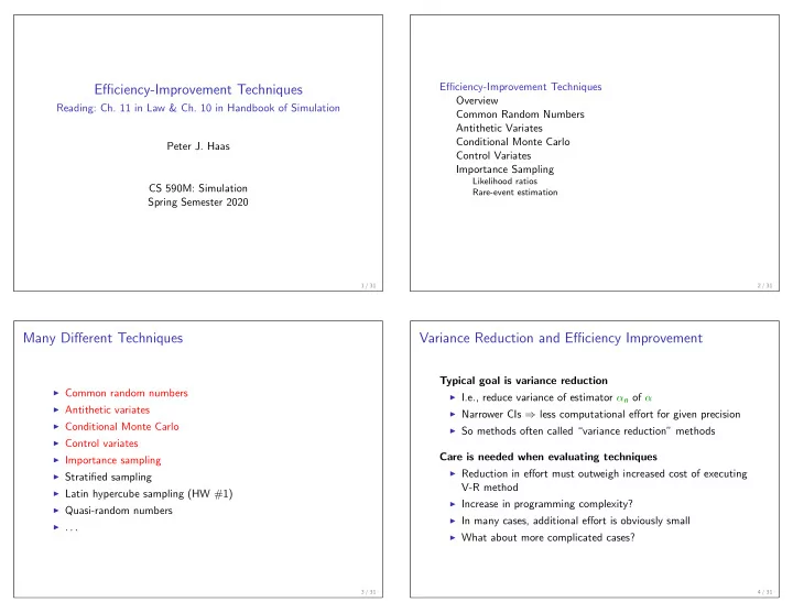
Efficiency-Improvement Techniques Efficiency-Improvement Techniques Overview Reading: Ch. 11 in Law & Ch. 10 in Handbook of Simulation Common Random Numbers Antithetic Variates Conditional Monte Carlo Peter J. Haas Control Variates Importance Sampling Likelihood ratios CS 590M: Simulation Rare-event estimation Spring Semester 2020 1 / 31 2 / 31 Many Different Techniques Variance Reduction and Efficiency Improvement Typical goal is variance reduction ◮ Common random numbers ◮ I.e., reduce variance of estimator α n of α ◮ Antithetic variates ◮ Narrower CIs ⇒ less computational effort for given precision ◮ Conditional Monte Carlo ◮ So methods often called “variance reduction” methods ◮ Control variates Care is needed when evaluating techniques ◮ Importance sampling ◮ Reduction in effort must outweigh increased cost of executing ◮ Stratified sampling V-R method ◮ Latin hypercube sampling (HW #1) ◮ Increase in programming complexity? ◮ Quasi-random numbers ◮ In many cases, additional effort is obviously small ◮ . . . ◮ What about more complicated cases? 3 / 31 4 / 31
Comparing Efficiency-Improvement Schemes Comparing Efficiency-Improvement Schemes, Continued Hammersley-Handscomb Efficiency Measure ◮ Can show: lim c →∞ N ( c ) / c = λ X a.s., where λ X = 1 / E [ τ X ] Trading off statistical and computational efficiency ◮ Hence ◮ Suppose α = E [ X ] = E [ Y ] N X ( c ) ⌊ λ X c ⌋ ◮ Should we generate i.i.d. replicates of X or Y to estimate α ? 1 1 � � α X ( c ) − α = X i − α ≈ X i − α N X ( c ) ⌊ λ X c ⌋ ◮ Assume large but fixed computer budget c i =1 i =1 ◮ Let τ X ( i ) be (random) time to generate X i � Var[ X ] 1 D � ∼ λ X c N (0 , 1) = √ c E [ τ X ] · Var[ X ] N (0 , 1) ◮ Assume that � � � � X 1 , τ X (1) , X 2 , τ X (2) , . . . are i.i.d. ◮ Number of X -observations generated within budget c is ◮ Similarly, N x ( c ) = max { n ≥ 0 : τ X (1) + · · · + τ X ( n ) ≤ c } � N X ( c ) 1 ◮ So estimator based on budget is α X ( c ) = X i 1 D N X ( c ) i =1 � √ c α Y ( c ) − α ∼ E [ τ Y ] · Var[ Y ] N (0 , 1) 1 ◮ Efficiency measure: E [ τ Y ] · Var[ Y ] (holds fairly generally) 5 / 31 6 / 31 Common Random Numbers (CRN) Applies when comparing alternate systems ◮ Intuition: Sharper comparisons if systems experience same Efficiency-Improvement Techniques random fluctuations Overview Common Random Numbers More precisely: Antithetic Variates ◮ Goal: Compare two perf. measures distributed as X and Y Conditional Monte Carlo ◮ Estimate α = E [ X ] − E [ Y ] = E [ X − Y ] Control Variates ◮ Generate i.i.d. pairs ( X 1 , Y 1 ) , . . . , ( X n , Y n ) Importance Sampling ◮ Point estimate: α n = (1 / n ) � n Likelihood ratios i =1 ( X i − Y i ) Rare-event estimation Var[ α n ] = 1 nVar [ X − Y ] = 1 � � Var[ X ] + Var[ Y ] − 2 Cov[ X , Y ] n ◮ So want Cov[ X , Y ] > 0 ◮ Note that Cov[ X , Y ] = 0 if X and Y simulated independently 7 / 31 8 / 31
CRN, Continued CRN, Continued Example: Long-run waiting times in two GI/G/1 queues Simple case: One random number per sample of X and of Y ◮ Suppose that ◮ Use same random number: X i = X i ( U i ) and Y i = Y i ( U i ) ◮ Interarrival times are i.i.d according to cdf G for both systems ◮ If X ( u ), Y ( u ) both ↑ (or both ↓ ) in u , then Cov[ X , Y ] > 0 ◮ Service times are i.i.d. according to cdf H i for queue i ( i = 1 , 2) ◮ True for inversion method: X i = F − 1 X ( U i ) and Y i = F − 1 Y ( U i ) ◮ Use one sequence ( U j : j ≥ 0) to generate a single stream of interarrival times for use in both systems In practice ◮ Use one sequence ( V j : j ≥ 0) to generate service times in ◮ Sync random numbers between systems as much as possible both systems: S 1 , j = H − 1 1 ( V j ) and S 2 , j = H − 1 2 ( V j ) for j ≥ 1 ◮ Use multiple random number streams, one per event ◮ Note: Need two streams { U i } and { V i } ◮ Jump-head facility of random number generator is crucial ◮ Systems get out of sync with only one stream 9 / 31 10 / 31 Antithetic Variates Applies when analyzing a single system ◮ Intuition: Combat “luck of the draw” by pairing each realized Efficiency-Improvement Techniques scenario with its opposite Overview Common Random Numbers More precisely: Antithetic Variates ◮ Goal: Estimate E [ X ] Conditional Monte Carlo ◮ Generate X 1 , . . . , X 2 n and set α n = ¯ X 2 n Control Variates ◮ Suppose pairs ( X 1 , X 2 ) , ( X 3 , X 4 ) , . . . , ( X 2 n − 1 , X 2 n ) are i.i.d. Importance Sampling (possible corr. within pairs) Likelihood ratios Rare-event estimation 1 � Var[ α 2 n ] = Var[ X 1 ] + · · · + Var[ X 2 n ] + 4 n 2 � 2 Cov[ X 1 , X 2 ] + · · · + 2 Cov[ X 2 n − 1 , X 2 n ] ◮ So want Cov[ X 2 j − 1 , X 2 j ] < 0 for j ≥ 1 11 / 31 12 / 31
Antithetic Variates, Continued Simple case: One random number per sample of X and of Y ◮ Use same random number: X i = X i ( U i ) and Y i = Y i (1 − U i ) ◮ If X ( u ), Y ( u ) both ↑ (or both ↓ ) in u , then Cov[ X , Y ] < 0 Efficiency-Improvement Techniques ◮ E.g., inversion method: X i = F − 1 X ( U i ) and Y i = F − 1 Overview Y (1 − U i ) Common Random Numbers Ex: Avg. waiting time of first 100 cust. in GI/G/1 queue Antithetic Variates Conditional Monte Carlo ◮ Interarrival times (service times) i.i.d according to cdf G ( H ) Control Variates ◮ Replication 2 k − 1: ( I j , S j ) = � G − 1 ( U j ) , H − 1 ( V j ) � Importance Sampling ◮ Replication 2 k : ( I j , S j ) = � G − 1 (1 − U j ) , H − 1 (1 − V j ) � Likelihood ratios Rare-event estimation Ex: Alternative method for GI/G/1 queue (Explain?) G − 1 ( U j ) , H − 1 ( V j ) ◮ Replication 2 k − 1: ( I j , S j ) = � � ◮ Replication 2 k : ( I j , S j ) = G − 1 ( V j ) , H − 1 ( U j ) � � Warning: CRN + AV together can backfire! [Law, p. 609] 13 / 31 14 / 31 Conditional Monte Carlo Conditional Monte Carlo, Continued Law of total expectation � � E E [ U | V ] = E [ U ] � � Example: Markovian GSMP X ( t ) : t ≥ 0 ◮ All events are simple w. exponential clock-setting dist’ns Variance decomposition ◮ Simulation algorithm (up to n th state transition time T n ) � � � � � � Var[ U ] = Var E [ U | V ] + E Var[ U | V ] ≥ Var E [ U | V ] D ◮ Generate states S 0 , . . . , S n − 1 ∼ DTMC w. transition matrix R D ◮ Generate holding time in each S k : H k � � ∼ exp λ ( S k ) Key Idea ◮ Goal: Estimate α = E [ Z ] with ◮ Simulate V and compute ˜ U = E [ U | V ] � T n du = � n − 1 � � Z = X ( u ) k =0 f ( S k ) H k f ◮ Then ˜ 0 U has same mean as U but smaller variance ◮ Variance reduction trick: ◮ So generate i.i.d replicates of ˜ U to estimate α = E [ U ] ◮ Generate states S 0 , . . . , S n − 1 as above Markovian GSMP example revisited ◮ Set holding time in S k = mean holding time = 1 /λ ( S k ) ◮ U = Z = � n − 1 k =0 f ( S k ) H k and V = ( S 0 , . . . , S n − 1 ) ◮ Q: Why does this work? ◮ So estimate E [ ˜ Z ] from i.i.d replicates ˜ Z 1 , . . . , ˜ Z m , where Z = E [ Z | S 0 , . . . , S n − 1 ] = � n − 1 k =0 f ( S k ) E [ H k | S k ] = � n − 1 ˜ 1 k =0 f ( S k ) λ ( S k ) 15 / 31 16 / 31
Control Variates Intuition: Exploit extra system knowledge ◮ Goal: Estimate α = E [ X ] Efficiency-Improvement Techniques ◮ Suppose that there exists a random variable Y such that Overview ◮ Y is strongly correlated with X Common Random Numbers ◮ E [ Y ] can be computed analytically Antithetic Variates ◮ Control variable: C = Y − E [ Y ] Conditional Monte Carlo ◮ Controlled estimator: X ( λ ) = X − λ C Control Variates ◮ E [ X ( λ )] = Importance Sampling ◮ v ( λ ) = Var[ X ( λ )] = Var[ X ] − 2 λ Cov[ X , C ] + λ 2 Var[ C ] Likelihood ratios Rare-event estimation ◮ v ( λ ) is minimized at λ ∗ = ◮ Minimizing variance is v ( λ ∗ ) = (1 − ρ 2 ) Var[ X ], where Cov[ X , C ] √ ρ = = correlation coefficient of X and C Var[ X ] · Var[ C ] 17 / 31 18 / 31 Control Variates, Continued Control Variates, Continued The method Internal and External Controls 1. Simulate i.i.d. pairs ( X 1 , C 1 ) , . . . , ( X n , C n ) ◮ C i in queueing example is an internal control, generated 2. Estimate λ ∗ by internally to the simulation ◮ Example of an external control: � 1 n n ◮ Simplify original simulation model M to a version M ′ where 1 λ ∗ � ( X i − ¯ � C 2 n = X n ) C i i performance measure α ′ can be computed analytically n − 1 n i =1 i =1 ◮ Generate replications of M and M ′ using common random numbers to obtain ( X 1 , X ′ 1 ) , . . . , ( X n , X ′ n ) 3. Apply usual estimation techniques to Z 1 , . . . , Z n , where ◮ Take C i = X ′ i − α ′ Z i = X i − λ ∗ C i for 1 ≤ i ≤ n Multiple controls Ex: E[avg delay] for first n customers in GI/G/1 queue ◮ X ( λ 1 , . . . , λ m ) = X − λ 1 C (1) − · · · − λ m C ( m ) ◮ X i = average delay in i th replication ◮ Can compute ( λ ∗ 1 , . . . , λ ∗ m ) by solving linear syst. of equations ◮ V i , k = k th service time in i replication, with E [ V i , k ] = 5 ◮ Essentially, we fit a linear regression model and simulate the ◮ Take C i = (1 / n ) � n k =1 V i , k − 5 leftover uncertainty (i.e., the residuals) ◮ Q: Why is this a good choice? 19 / 31 20 / 31
Recommend
More recommend
Explore More Topics
Stay informed with curated content and fresh updates.


