Effective resistance of random trees G abor Lugosi ICREA and - PowerPoint PPT Presentation

Effective resistance of random trees G´ abor Lugosi ICREA and Pompeu Fabra University, Barcleona, Spain joint work with Louiiiiiiigi Addario-Berry (Oxford, UK) Nicolas Broutin (INRIA, France),

electric networks An electric network is a connected graph G = (V , E) . Each edge e ∈ E is equipped with a resistance r e ≥ 0 . c e = 1 / r e is the conductance of e . Let A , B ⊂ V and assign “voltage” U(u) = 1 to each u ∈ A and U(v) = 0 for all v ∈ B . U can be extended, in a unique way, to all vertices according to Ohm’s law and Kirchhoff’s node law .

electric networks Given u , v ∈ V joined by e ∈ E , the current from u to v is i(u , v) . By Ohm’s law, i(u , v)r e = U(u) − U(v) . ∈ A ∪ B , � By Kirchhoff’s node law, for any u / v:v ∼ u i(u , v) = 0 . The effective conductance between A and B is � � C(A ↔ B) = i(u , v) . v:v ∼ u u ∈ A The effective resistance between A and B is R(A ↔ B) = 1 / C(A ↔ B) .

equivalent transformations r r' r +r' = c c+c' = c'

connection to random walks A random walk on G . At each vertex, transition probabilities are proportional to conductances. Starting the walk at vertex v , the probability that the walk reaches A before B is exactly U(v) . Helpful for studying transience/recurrence of random walks on infinite graphs. Doyle and Snell (1984), Lyons and Peres (2008+).

random electrical networs Benjamini and Rossignol (2007) study electrical networks with random resistances. The r e are i.i.d. taking values in [a , b] with 0 < a < b < ∞ . They study, in Z d , the effective resistance between the origin and the boundary of a centered box of side n .

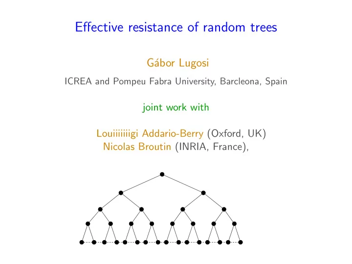
random trees We consider the rooted complete binary tree of height n . The resistance of an edge at depth d is r e = 2 d X e where the X e are i.i.d. taking values in [a , b] . The scaling corresponds to the critical case. See Pemantle (1988), Lyons (1990), Lyons and Pemantle (1992) for related models of random walks.

main results Let R n and C n be the resistance and conductance between the root and the set of vertices at depth n . Let µ = E X e and σ 2 = var (X e ) . E R n = µ n − σ 2 µ ln n + O(1) and var (R n ) = O(1) µ n + σ 2 E C n = 1 µ 3 · ln n n 2 + O(n − 2 ) var (C n ) = O(n − 4 ) and

proof ideas The key is to establish the concentration results first, starting with the conductance. Decompose the tree into two T n parallel subtrees. T ′ n − 1 The subtrees are rooted at an T n − 1 edge instead of a vertex.

Efron-Stein inequality If X 1 , . . . , X n are independent random variables and f : R n → R then var (f(X 1 , . . . , X n )) n 1 �� � 2 � � f(X 1 , . . . , X n ) − f(X 1 , . . . , X ′ ≤ E i , . . . , X n ) 2 i=1

the variance of the conductance We write the conductance as a function of 3 independent random variables. C 1 C n = C 1 (C n , 1 + C n , 2 ) C 1 + C n , 1 + C n , 2 C n, 1 C n, 2 Now use Efron-Stein. This leads to the recursion var (C n ) ≤ 1 K 2 var (C n − 1 )+ (n − 1) 4

the variance of the resistance We have var (C n ) = O(n − 4 ) . �� 1 � �� E C n � � � � � � � P � R n − � > t = P − 1 � > t E C n � � � � E C n C n � � t � ≤ P | C n − E C n | > b 2 n 2 K ≤ t 2 This implies �� � 2 � 1 var (R n ) ≤ E R n − = O(1) E C n

the expected conductance and resistance Once again we work with the recursion C n = C 1 (C n , 1 + C n , 2 ) C 1 + C n , 1 + C n , 2 The variance bound is crucial.

flows A unit flow is a function Θ over the edges { (u , v) : u ∼ v } which is • antisymmetric: Θ(u , v) = − Θ(v , u) , • � v:v ∼ u Θ(u , v) = 0 for any u / ∈ A ∪ B , • � � � � Θ(u , v) = Θ(u , v) = 1 . u ∈ A v / ∈ A:v ∼ u v ∈ B u / ∈ B:u ∼ v Thomson’s principle : � r e Θ(e) 2 R(A ↔ B) = inf Θ e ∈ E The unique flow Θ ∗ which attains the infimum is the current i(u , v) .

an alternative approach By Efron-Stein we get var (R n ) ≤ (b − a) 2 � Θ ∗ (e) 4 � � 2 2d(e) E . 2 e ∈ E(T n ) If e 0 , . . . , e n − 1 are the edges on the leftmost branch, n − 1 var (R n ) ≤ (b − a) 2 � Θ ∗ (e i ) 4 � � 2 3i E , 2 i=0 Also, R r n , i Θ ∗ (e i ) = Θ ∗ (e i − 1 ) · . R ℓ n , i + R r n , i With this technique and generalizations of Efron-Stein we can prove � (R n − E R n ) k � E = O(1) for all k .

questions • More general trees? • Galton-Watson trees. Scale by expected number of offspring E B . • If Z n is the number of vertices at depth n and W = lim n Z n / ( E B) n , is it true that R n n → µ W?