EEEEKKKKK!!!! In January, 1942 a Soviet Ilyushin 4 flown by - - PowerPoint PPT Presentation

EEEEKKKKK!!!!

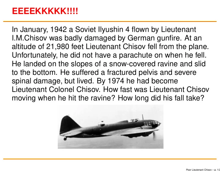
In January, 1942 a Soviet Ilyushin 4 flown by Lieutenant I.M.Chisov was badly damaged by German gunfire. At an altitude of 21,980 feet Lieutenant Chisov fell from the plane. Unfortunately, he did not have a parachute on when he fell. He landed on the slopes of a snow-covered ravine and slid to the bottom. He suffered a fractured pelvis and severe spinal damage, but lived. By 1974 he had become Lieutenant Colonel Chisov. How fast was Lieutenant Chisov moving when he hit the ravine? How long did his fall take?

Poor Lieutenant Chisov – p. 1/2

The Drag Force

| Ff| = 1 2 DρAv2 D - drag coefficient (dimen- sionless). ρ - air density (kg/m3). A - Cross sectional area (m2). v - speed (m/s).

2007-12-13 17:51:17

(m/s)

t

v 0.5 1 1.5 2 2.5 3 3.5 4 Resistive Force (N) 0.02 0.04 0.06 0.08 0.1 0.12 0.14 0.16 0.18

/ ndf

2

χ 0.0001598 / 10 p0 ± p1 ± p2 0.0002145 ± 0.01589 / ndf

2

χ 0.0001598 / 10 p0 ± p1 ± p2 0.0002145 ± 0.01589

Resistive Force on Coffee Filters

Poor Lieutenant Chisov – p. 2/2

The Drag Force

Aerodynamic forces acting on an artillery shell. The force W is the drag or air resistive force, La is the lift, Fg is gravity, and the point D is the center

• f pressure. Note the change in the air resistive force at the speed of

sound.

Poor Lieutenant Chisov – p. 3/2

Resistive Force on a Baseball

Jonathan Papelbon gives Derek Jeter some chin music at 90 mph (40 m/s). What is the drag coefficient of a baseball? What is the resistive force at that speed? The mass of a baseball is 0.145 kg, its radius is 3.7 cm, and its terminal velocity is measured to be 43 m/s.

Poor Lieutenant Chisov – p. 4/2

Approximating a Function

The plot below shows an arbitrary curve (black) with the tangent curve (red) at one point.

a x 1 2 3 4 5 100 200 300 400 x yfx

Poor Lieutenant Chisov – p. 5/2

Taylor Series for the Sine function

The plot below shows the sine function. What are the first two nonzero terms of the Taylor series for the sine function expanded about the point θ = 0? How close do they come to the sine function?

(radians) θ 5 10 15 20 25 30 (radians) θ 5 10 15 20 25 30 ) θ sin(

• 1
• 0.5

0.5 1

Poor Lieutenant Chisov – p. 6/2

Taylor Series for the Sine function

(radians) θ 5 10 15 20 25 30 (radians) θ 5 10 15 20 25 30 ) θ sin(

• 1
• 0.5

0.5 1

Taylor Series of order 3 Sine function

(radians) θ 0.5 1 1.5 2 2.5 3 (radians) θ 0.5 1 1.5 2 2.5 3 ) θ sin(

• 1
• 0.5

0.5 1

Taylor Series of Third Order Sine function

Poor Lieutenant Chisov – p. 7/2

The Integral Convergence Test

200 400 600 800 1000 1200 2 4 6 8 xn fx

• m1

n

• 1

m versus lnx

Poor Lieutenant Chisov – p. 8/2

Numerical Differentiation of a Curve

f(x) x

x x x x x x

1 2 3 −1 −2 −3

x

h

f f f f f

−3 −2 2 3 1

A Computer Curve

f

−1

f0

h

Poor Lieutenant Chisov – p. 9/2

Numerical Differentiation of a Curve

f(x) x

x x x x x x

1 2 3 −1 −2 −3

x

h

f f f f f

−3 −2 2 3 1

A Computer Curve

f

−1

f0

h

Poor Lieutenant Chisov – p. 10/2

Numerical Differentiation of a Curve

f(x) x

x x x x x x

1 2 3 −1 −2 −3

x

h

f f f f f

−3 −2 2 3 1

A Computer Curve

f

−1

f0

h

Poor Lieutenant Chisov – p. 11/2

Life is a Differential Equation (DE)

Some definitions first

Ordinary DE One independent variable; only total derivatives.

Poor Lieutenant Chisov – p. 12/2

Life is a Differential Equation (DE)

Some definitions first

Ordinary DE One independent variable; only total derivatives. Partial DE More than one variable so use partial derivatives.

Poor Lieutenant Chisov – p. 12/2

Life is a Differential Equation (DE)

Some definitions first

Ordinary DE One independent variable; only total derivatives. Partial DE More than one variable so use partial derivatives. Order of the DE Highest derivative in the DE.

Poor Lieutenant Chisov – p. 12/2

Life is a Differential Equation (DE)

Some definitions first

Ordinary DE One independent variable; only total derivatives. Partial DE More than one variable so use partial derivatives. Order of the DE Highest derivative in the DE. Degree of the DE Power of the highest order derivative in the DE.

Poor Lieutenant Chisov – p. 12/2

Life is a Differential Equation (DE)

Some definitions first

Ordinary DE One independent variable; only total derivatives. Partial DE More than one variable so use partial derivatives. Order of the DE Highest derivative in the DE. Degree of the DE Power of the highest order derivative in the DE. Linear DE No multiplications among dependent variables and their derivatives.

Poor Lieutenant Chisov – p. 12/2

Life is a Differential Equation (DE)

Some definitions first

Ordinary DE One independent variable; only total derivatives. Partial DE More than one variable so use partial derivatives. Order of the DE Highest derivative in the DE. Degree of the DE Power of the highest order derivative in the DE. Linear DE No multiplications among dependent variables and their derivatives. Homogeneous Every single term contains the dependent variables

• r their derivatives.

Poor Lieutenant Chisov – p. 12/2

Life is a Differential Equation (DE)

Some definitions first

Ordinary DE One independent variable; only total derivatives. Partial DE More than one variable so use partial derivatives. Order of the DE Highest derivative in the DE. Degree of the DE Power of the highest order derivative in the DE. Linear DE No multiplications among dependent variables and their derivatives. Homogeneous Every single term contains the dependent variables

• r their derivatives.

General Solution Results of integrating the DE; nth order DE require n conditions to fix all the constants.

Poor Lieutenant Chisov – p. 12/2

Life is a Differential Equation (DE)

Some definitions first

Ordinary DE One independent variable; only total derivatives. Partial DE More than one variable so use partial derivatives. Order of the DE Highest derivative in the DE. Degree of the DE Power of the highest order derivative in the DE. Linear DE No multiplications among dependent variables and their derivatives. Homogeneous Every single term contains the dependent variables

• r their derivatives.

General Solution Results of integrating the DE; nth order DE require n conditions to fix all the constants. Particular Solution General solution plus the n conditions.

Poor Lieutenant Chisov – p. 12/2

Life is a Differential Equation (DE)

Some definitions first

Ordinary DE One independent variable; only total derivatives. Partial DE More than one variable so use partial derivatives. Order of the DE Highest derivative in the DE. Degree of the DE Power of the highest order derivative in the DE. Linear DE No multiplications among dependent variables and their derivatives. Homogeneous Every single term contains the dependent variables

• r their derivatives.

General Solution Results of integrating the DE; nth order DE require n conditions to fix all the constants. Particular Solution General solution plus the n conditions. Initial Value Problem Find v(t) and y(t) when v(t0) = v0 or y(t0) = y0.

Poor Lieutenant Chisov – p. 12/2

Solving First-Order, Ordinary DEs

• 1. The differential equation and the initial conditions are
• given. For example

dy dt = f(t, y) and y(t0) = y0

and y(t1) is unknown.

• 2. Divide the range [t0, t1] into pieces.
• 3. Generate a recursion relationship between adjacent

points.

• 4. Perform a step-by-step integration.

Poor Lieutenant Chisov – p. 13/2

Nuclear Decay

The rate of radioactive decay of atomic nuclei is proportional to the number of nuclei N in the sample so

dN dt = −λN

where λ is a constant of proportionality (related to the half-life) and the negative sign means the number of nuclei is decreasing. The initial condition is N(t = 0) = N0 = 1000.

• 1. Write down the analytical solution.
• 2. Generate an algorithm to solve this differential equation

and apply it for the first three values of N(t) ‘by hand’ for

h = ∆t = 0.1 s and λ = 0.2 s−1.

• 3. Find the solution for the first sixty seconds.

Poor Lieutenant Chisov – p. 14/2

Nuclear Decay Results

t(s) Calculation Result Analytic Result

Poor Lieutenant Chisov – p. 15/2

Solution of dN

dt = −λN using an Euler algorithm

(* initial parameter values *) N0 = 1000.0; lambda = 0.2; t0 = 0.0; t1 = 60.0; h = 0.1; (* starting point of recursion relationship. *) Nn = N0; (* make the table *) table1 = Table[ {t, Nplus = Nn*(1 - lambda*h); Nn = Nplus }, {t, t0 + h, t1, h}]; (* stick the starting point at the front of the table. *) table1 = Prepend[table1, {t0, N0}]; Results t (s) N 0.0 1000.0 0.1 980.0 0.2 960.4 0.3 941.2

10 20 30 40 50 60 ts 200 400 600 800 1000 N

Poor Lieutenant Chisov – p. 16/2

The Limits of Accuracy

• 1. Consider the following code fragment. Why does a = b?

a = 1.0*10ˆ17 + 1.0 - 1.0*10ˆ17; b = 1*10ˆ17 + 1 - 1*10ˆ17; Print["a=", a, " b=", b] a=0. b=1

• 2. Consider the following function.

∆ = cos θ−sin(θ + h) − sin(θ − h) 2h The plot shows the dependence

• f the function on the stepsize h.

0.00001 0.00003 0.00007 51012 11011 51011 11010 51010 1109 h

• Limits of Accuracy

Poor Lieutenant Chisov – p. 17/2

PROBLEMS!!!!!!

Original initial conditions.

20 40 60 80 100 120 80 60 40 20 t s v ms Velocity of Lieutenant Chisov 20 40 60 80 100 120 1000 2000 3000 4000 5000 6000 7000 ts ym Altitude of Lieutenant Chisov

Increase the initial altitude.

Poor Lieutenant Chisov – p. 18/2

PROBLEMS!!!!!!

Original initial conditions.

20 40 60 80 100 120 80 60 40 20 t s v ms Velocity of Lieutenant Chisov 20 40 60 80 100 120 1000 2000 3000 4000 5000 6000 7000 ts ym Altitude of Lieutenant Chisov

Increase the initial altitude.

50 100 150 80 60 40 20 t s v ms Velocity of Lieutenant Chisov 50 100 150 2000 4000 6000 8000 10000 12000 ts ym Altitude of Lieutenant Chisov

Poor Lieutenant Chisov – p. 18/2

The Stability Problem

Red v Blue v 10 20 30 40 50 1.0 0.5 0.0 0.5 1.0 n v

Poor Lieutenant Chisov – p. 19/2

SOLUTIONS!!!!!!

Increase the initial altitude.

50 100 150 80 60 40 20 t s v ms Velocity of Lieutenant Chisov 50 100 150 2000 4000 6000 8000 10000 12000 ts ym Altitude of Lieutenant Chisov

The fix is in.

50 100 150 80 60 40 20 ts v ms Velocity of Lieutenant Chisov 50 100 150 2000 4000 6000 8000 10000 12000 t s x m Velocity of Lieutenant Chisov

Poor Lieutenant Chisov – p. 20/2

The Harmonic Oscillator - Stating the Problem

Hooke’s Law states that Fs = −kx where Fs is the force exerted by a spring (the restoring force) and x is the displacement from equi- librium where there is no net force acting on the mass.

• 1. What differential equation does x satisfy?
• 2. What is the solution?
• 3. How would you test the solution?
• 4. What is the physical meaning of the constants in the solution?

Poor Lieutenant Chisov – p. 21/2

The Harmonic Oscillator - The Solution

The solution for Hooke’s Law is

x(t) = A cos(ωt + φ)

where x(t) is the displacement from equilibrium.

t 1 2 3 4 5 6 7 8 9 10 x(t)

• 1
• 0.5

0.5 1 A Cosine Curve

Period Amplitude Phase

Poor Lieutenant Chisov – p. 22/2

The Simple Harmonic Oscillator - An Example

A harmonic oscillator consists of a block of mass m = 0.33 kg attached to a spring with spring constant k = 400 N/m. See the figure below. At time t = 0.0 s the block’s displacement from equi- librium and its velocity are y =

0.100 m and v = −13.6 m/s. (1)

Find the particular solution for this oscillator. (2) Use a centered derivative formula to generate an algorithm for solving the equation

• f motion.
• Poor Lieutenant Chisov – p. 23/2

The Pendulum - Stating the Problem

Hooke’s Law states that Fs = −kx where Fs is the force exerted by a spring (the restoring force) and x is the displace- ment from equilibrium where there is no net force acting on the mass. One can show the similarity between the simple pendulum and the harmonic oscillator.

• 1. What differential equation does θ

satisfy for small angles?

• 2. What is the solution?
• 3. How would you test the solution?

m mgsin mgcos θ θ θ C g L O

Poor Lieutenant Chisov – p. 24/2

The Simple Pendulum with Friction

Consider the simple pendulum shown here. What is the differential equation describing the motion when the following forces are included in addition to gravity? For friction use Ffriction = − q Lv where q is a constant specific to a partic- ular body. For the driving force use Fdriving = FD sin(Ωt) where FD is the magnitude of the driving force and Ω is its angular frequency. m mgsin mgcos θ θ θ C g L O

Poor Lieutenant Chisov – p. 25/2

The Physical Pendulum

Consider the rod rotating about an end point in the figure. Starting from the defi- nition of the torque τ = r × F, (1) derive the differential equation the an- gular position θ must satisfy. (2) Derive a new differential equation if the pendulum is damped by a friction force Ff = −b v where b is some constant describing the the pendulum. (3) Derive a final differential equation if the pendulum is now also driven by a force Fdrive = FD sin(Ωt)ˆ θ. (4) What does the phase space look like for each set of conditions if the initial con- ditions are θ0 = 25◦ and ω0 = 0 rad/s? m mgsin L cm θ g θ O C mgcosθ

Poor Lieutenant Chisov – p. 26/2

Harmonic Oscillator With Coupled Equations - 1

(* Solving the mass on a spring problem. Initial conditions and parameters *) x0 = 0.0; (* initial position in meters *) v0 = 2.0; (* initial velocity in m/s *) t0 = 0.0; (* initial time in seconds *) (* set up the first two points. step size *) step = 0.1; t1 = t0 + step; x1 = x0 + v0*step; v1 = v0 - ( step*kspring*x0/mass); xminus = x0; (* initial value of x *) vminus = v0; (* initial value of v *) xmid = x1; vmid = v1; mass = 0.33; (* the mass in kg *) kspring = 0.5; (* spring constant in N/m *)

Poor Lieutenant Chisov – p. 27/2

Harmonic Oscillator With Coupled Equations - 2

(* limits of the iterations. since we already have y(t=0) and we have calculated y(t=step), then the first value in the table will be for t=2*step. *) tmin = 2*step; tmax = 25.0; (* create a table of ordered (t,x). for each component the next value is calculated and then variables are incremented for the next interation. tpos = Table[ {t, vplus = vminus - (2*step*kspring/mass)*xmid; xplus = xminus + (2*step*vmid); vminus = vmid; vmid = vplus; xminus = xmid; xmid = xplus }, {t, tmin, tmax, step} ];

Poor Lieutenant Chisov – p. 28/2