Gaussian kernel regression as an improved estimator for - PowerPoint PPT Presentation

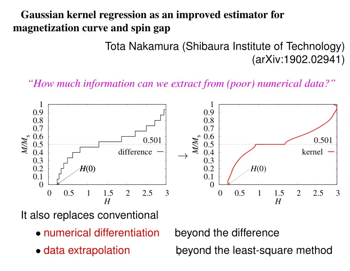
Gaussian kernel regression as an improved estimator for magnetization curve and spin gap Tota Nakamura (Shibaura Institute of Technology) (arXiv:1902.02941) “How much information can we extract from (poor) numerical data?” 1 1 0.9 0.9 0.8 0.8 0.7 0.7 0.6 0.6 M/M s M/M s 0.501 0.501 0.5 0.5 difference kernel 0.4 0.4 → 0.3 0.3 0.2 H (0) H (0) 0.2 H (0) 0.1 0.1 0 0 0 0.5 1 1.5 2 2.5 3 0 0.5 1 1.5 2 2.5 3 H H It also replaces conventional • numerical differentiation beyond the difference • data extrapolation beyond the least-square method 1

Outline 1. The Gaussian kernel regression and the Bayesian inference 2. Magnetization curve (a) S = 1 / 2 bond-alternation XY spin chain (b) kagome antiferromagnet 3. Spin gap and the size extrapolation 2

§ 1. The Gaussian kernel regression and the Bayesian inference (Problem) Obtain a model function y = F ( x ) for data x i , y i , and ∆ y i 0.24 data model function 0.23 y 0.22 0.21 0 0.02 0.04 0.06 0.08 x (Answer) F ( x ) = d ij K ( x i , x ) C − 1 ij y j � with K ( x i , x ) : Gauss kernel function C ij : covariance matrix of data 3

§ 1. The Gaussian kernel regression and the Bayesian inference Recipe 1. Define a covariance matrix C ij ( i, j = 1 , · · · d ) C ij = (∆ y i ) 2 δ ij + K ( x i , x j ) with a Gaussian kernel function  − ( x i − x j ) 2   K ( x i , x j ) = θ 2  + θ 2   1 exp ( x i � = x j )     3 2 θ 2     2 2. Calculate determinant and inverse of C 3. Find ( θ 1 , θ 2 , θ 3 ) that maximize the log-likelihood function log L ( θ 1 , θ 2 , θ 3 ) = − 1 1 2 y i C − 1 2 log | C | − ij y j � ij 4. Using ( θ 1 , θ 2 , θ 3 ), C − 1 ij , and data ( x i , y i ) , F ( x ) = d ij K ( x i , x ) C − 1 ij y j � This is analytically differentiable! 4

§ 1. The Gaussian kernel regression and the Bayesian inference Bayesian inference in the scaling analysis of critical phenomena K. Harada, PRE 84, 056704 (2011) • Include unknown parameters, T c and ν , in x i and y i x i = (1 /T − 1 /T c )( L/ 256) 1 /ν y i = U ( T, L ) (Binder ratio) • Find ( T c , ν ) and ( θ 1 , θ 2 , θ 3 ) that maximize log L 5

§ 1. The Gaussian kernel regression and the Bayesian inference 1. obtain analytically-differentiable model function ↓ improves numerical differentiation → magnetization curve by H ( M ) = ∂E ( M ) ∂M 2. estimate unknown parameters if included in ( x i , y i ) ↓ improves data extrapolation → plateau magnetization → spin gap → extrapolation of N → ∞ 6

Outline 1. The Gaussian kernel regression and the Bayesian inference 2. Magnetization curve 3. Spin gap and the size extrapolation 4. Other applications 7

§ 2 Magnetization curve :Recipe for a standard numerical evaluation 1. Calculate the ground state energy E ( M ) 2. Estimate H such that E − HM is minimum ↔ H ( M ) = ∂E ( M ) by the difference ∂M 8

§ 2 Magnetization curve :Recipe for the kernel method 1. We have E ( M ) of ∆ -chain with 30 spins by using Titpack ver2 original data 0.4 0.2 0 E/N -0.2 -0.4 -0.6 -0.8 -1 0 0.2 0.4 0.6 0.8 1 M/M s 9

§ 2 Magnetization curve :Recipe for the kernel method 2. Assume a plateau point ( M p , E ( M p )) and divide data at M p original data 0.4 0.2 0 E/N -0.2 -0.4 plateau point (trial) -0.6 -0.8 -1 0 0.2 0.4 0.6 0.8 1 M/M s 10

§ 2 Magnetization curve :Recipe for the kernel method 3. Define mirror data with respect to the plateau point original data 0.4 mirror data 0.2 0 E/N -0.2 -0.4 plateau point (trial) -0.6 -0.8 -1 0 0.2 0.4 0.6 0.8 1 M/M s Now, x i and y i include M p and E ( M p ) . 11

§ 2 Magnetization curve :Recipe for the kernel method 4. Obtain the model function by the kernel method original data 0.4 mirror data 0.2 0 model functions E/N -0.2 -0.4 plateau point (trial) -0.6 -0.8 -1 0 0.2 0.4 0.6 0.8 1 M/M s bad guess gives a non-smooth function: low value of log L 12

§ 2 Magnetization curve :Recipe for the kernel method 5. Find a plateau point that gives the largest log L 18 16 14 log L 12 10 all(800) 8 select(80) 6 0.4 0.45 0.5 0.55 0.6 M p 13

§ 2 Magnetization curve :Recipe for the kernel method 6. Final result original data 0.4 mirror data 0.2 0 model functions E/N -0.2 plateau point -0.4 (final) -0.6 (0.5015,-0.2546) -0.8 -1 0 0.2 0.4 0.6 0.8 1 M/M s differentiable function of E(M) is now obtained 14

§ 2 Magnetization curve :Recipe for the kernel method 7. The magnetization curve is obtained by H ( M ) = ∂E ( M ) ∂M 1 0.9 (b) 0.8 0.7 0.6 M/M s 0.501 0.5 kernel(0.4< M p <0.6) 0.4 kernel( M p =0) 0.3 0.2 kernel( M p =1) 0.1 difference 0 0 0.5 1 1.5 2 2.5 3 H 15

§ 2 Magnetization curve :Compare with exact results S = 1 / 2 Bond-alternation XY chain with 30 spins 1 kernel exact 0.8 difference 0.6 1+λ 1+λ 1+λ M/M s 1−λ 1−λ 1−λ 0.4 λ =0.1 0.2 λ =0.5 λ =0.3 0 0 0.2 0.4 0.6 0.8 1 H we set M p = 0 16

§ 2 Magnetization curve :kagome antiferromagnet Using mixed data of 30 spins and 27 spins 1 kernel difference 0.8 DMRG 0.6 M/M s 0.4 0.2 (b) 0 0 0.5 1 1.5 2 2.5 3 H we set M p = 0 , 1 / 9 , 1 / 3 , 5 / 9 , 7 / 9 DMRG(Nishimoto et al. 2013) 17

Outline 0. Motivation 1. The Gaussian kernel regression and the Bayesian inference 2. Magnetization curve 3. Spin gap and the size extrapolation 4. Other applications 18

§ 3 Spin gap Critical field H (0) is another definition for the spin gap 1 0.9 0.8 0.7 0.6 M/M s 0.501 -0.26 0.5 N =30 26 kernel -0.28 0.4 model function -0.3 0.3 E/N -0.32 0.2 H (0) 0.1 -0.34 0 -0.36 0 0.5 1 1.5 2 2.5 3 -0.38 0 0.1 0.2 0.3 0.4 0.5 H M/M s 19

§ 3 Spin gap : S = 1 / 2 bond-alternation XY model, λ = 0 . 1 case 0.16 0.14 0.12 Spin Gap 0.1 λ =0.1 0.08 0.06 H (0) E (1)- E (0) 0.04 Model 0.02 (b) Least-sq 0 0 0.02 0.04 0.06 0.08 1/ N exact gap is 0.1 Spin gap( N = ∞ )=0.0995(1) 20

§ 3 Spin gap :kagome antiferromagnet 0.3 E (1)- E (0)[PBC] E (1)- E (0)[TBC] 0.25 H (0)[PBC] H (0)[TBC] 0.2 Spin Gap Model 0.15 0.1 0.05 (a) 0 0 0.01 0.02 0.03 0.04 0.05 1/ N PBC: periodic boundary condition TBC: twisted boundary condition Spin gap( N = ∞ )=0.0276(2) 21

§ 3 Spin gap :Tips ”Cross Validation by random noise works fine” ∆ -chain case 0.27 0.23 H (0) over fitting Spin gap( N = ∞ ) E (1)- E (0) 0.26 optimal with CV noiseful 0.225 0.25 without CV Spin Gap noiseful 0.24 0.22 0.23 0.22 0.215 0.21 10 -6 10 -5 10 -4 10 -3 10 -2 0 0.02 0.04 0.06 0.08 1/ N eff ∆ E(M) Search parameters by data with a noise Validate the results(calculate log L ) by data with another noise 22

Summary • We can extract more physical information by using the kernel method. • It replaces numerical differentiation and data extrapolation. • Finite but small spin gap in kagome antiferromagnet • We cannot use machine learning as a black box – No-Free-Lunch theorem: we need some extra tips – There is no “grand truth”: it works well when it works 23