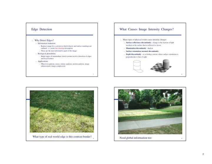
edge detection what causes image intensity changes
play

Edge Detection What Causes Image Intensity Changes? Many types - PowerPoint PPT Presentation

Edge Detection What Causes Image Intensity Changes? Many types of physical events cause intensity changes l l Why Detect Edges? u Surface reflectance discontinuity - change in the fraction of light u Information reduction incident on the


  1. Edge Detection What Causes Image Intensity Changes? Many types of physical events cause intensity changes l l Why Detect Edges? u Surface reflectance discontinuity - change in the fraction of light u Information reduction incident on the surface that is reflected to viewer l Replace image by a cartoon in which objects and surface markings are outlined ⇒ create line drawing description u Illumination discontinuity - shadow l These are the most informative parts of the image u Surface orientation (normal) discontinuity u Biological plausibility u Depth discontinuity - at occluding contour, where surface orientation is l Initial stages of mammalian vision systems involve detection of edges perpendicular to line of sight and local features u Applications l Object recognition, stereo, texture analysis, motion analysis, image enhancement, image compression 1 2 What type of real-world edge is this contrast border? Need global information too 3 4 1

  2. What Does an Edge Look Like? l Step l Ramp l Roof l Line (bar) 5 6 coarse scale, fine scale high high threshold threshold 7 8 2

  3. Edge Detectors in the HVS coarse scale Simple (border) low threshold Complex l Sum activity from an array of oriented simple cells 9 10 Orientation Columns in V1 Craik-O’Brien-Cornsweet Illusion l A “hypercolum” = complete set of orientations 11 12 3

  4. Luminance Differences Affect our Perceptions Koffka Ring l Artists use the technique of “equiluminance” to blur outlines and suggest motion . We cannot perceive the edges of objects where object and background have the same luminance. If parts of a painting are equiluminant, their positions become ambiguous. They may seem to shift position or to float l Equiluminant colors have special properties, e.g., they can make a painting appear unstable 13 14 Detail from Richard Anuszkiewicz’s Plus Reversed , 1960 Equiluminant Colors l An object that can be seen by both subdivisions of the visual system will be perceived accurately. But if the two subdivisions are not balanced in their response to an object, it may look peculiar. l For example, an object defined by equiluminant colors can be seen by the What system but is invisible (or poorly seen) by the Where system. It may seem flat, it may seem to shift position, or it may seem to float ambiguously because there is too little luminance contrast to provide adequate information about its three-dimensional shape, its location in space, or its motion (or lack of it). l Conversely, something defined by very low contrast contours is seen by the Where system but not the What system and may seem to have depth and spatial organization but no clear shape. ������������������������������������������������������������������ 15 16 4

  5. Edge Detection Goals Edge Operator Properties l Shift invariant (translation invariant, position invariant) l Good detection : Low false alarm rate and low false u If g(x,y) = Op[f(x,y)] then g(x-a, y-b) = Op[f(x-a, y-b)] dismissal rate ⇒ maximize signal-to-noise (S/N) ratio l Isotropic (rotation invariant) vs. non-isotropic l Good localization : Mark point closest to “center” of true l Derivative order (if differentiation-based method) edge ⇒ minimize distance between marked point and l Linear vs. non-linear center u Op[a f 1 (x,y) + b f 2 (x,y)] = a Op[f 1 (x,y)] + b Op[f 2 (x,y)] = a g 1 (x,y) + b g 2 (x,y) l Uniqueness : Only one response to a single edge l Scale (operator neighborhood size) l Good property measurement : Orientation, contrast, etc. u g(x,y) = Op[f(x+a, y+b), ∀ -k < a, b < k ] l Convolution (linear and shift-invariant) 17 18 Edge and Local Feature Detection Methods 1D Edge Detection l An ideal edge is a step function l Gradient-based edge detection l Edge detection by function fitting I (x) l Second derivative edge detectors l Edge linking and the construction of the chain graph x I ′ (x) x 19 20 5

  6. 1D Edge Detection 1D Edge Detection I ′′ (x) l More realistically, image edges are blurred and the regions that meet at those edges have noise or variations in intensity u Blur - high first derivatives near edges x u Noise - high first derivatives within regions that meet at edges I ′ (x) I (x) l The first derivative of I (x) has a peak at the edge l The second derivative of I (x) has a zero crossing at the edge x x 21 22 Edge Detection in 2D Computing First Derivative l To compute first derivative in direction θ , calculate from l Let I (x,y) be the image intensity function. It has linear combination of derivatives from any two derivatives in all directions non-collinear directions u ∂ I ( x , y )/ ∂ x = lim I ( x + ∆ x , y ) - I ( x , y ) / ∆ x ≈ I ( u +1, v ) - I ( u,v ) � x = x ′ cos θ - y ′ sin θ u Gradient of I (x, y) is a vector ∇ ∇ I (x, y) = [ ∂ I / ∂ x, ∂ I / ∂ y] T specifying ∇ ∇ y = x ′ sin θ + y ′ cos θ y y ′ x ′ the direction of greatest rate of change in intensity (i.e., ∂ I / ∂ x ′ = ∂ I / ∂ x ∂ x/ ∂ x ′ + ∂ I / ∂ y ∂ y/ ∂ y ′ � = ∂ I / ∂ x cos θ + ∂ I / ∂ y sin θ perpendicular to the edge’s direction) θ ∂ I / ∂ y ′ = - ∂ I / ∂ x sin θ + ∂ I / ∂ y cos θ x u From gradient can determine the direction in which the first � ( ∂ I / ∂ x ′ ) 2 + ( ∂ I / ∂ y ′ ) 2 = ( ∂ I / ∂ x) 2 + ( ∂ I / ∂ y) 2 derivative is highest, and the magnitude of the first derivative in � So, sum of squares of first derivative is that direction isotropic, non-linear u Magnitude = [( ∂ I / ∂ x) 2 + ( ∂ I / ∂ y) 2 ] 1/2 � Similarly, all derivatives of odd ordcr raised to an even power are isotropic u Direction = tan -1 ( ∂ I / ∂ y)/( ∂ I / ∂ x) 23 24 6

  7. Gradient Edge Detection in 2D l With a digital image, the partial derivatives are replaced by l Gradient = [ ∂ I / ∂ x, ∂ I / ∂ y] T finite differences: v l What direction is first derivative a maximum? u ∆ x I = I (u+1, v) - I (u, v) u Set ∂ / ∂θ ( ∂ I / ∂ x ′ ) = 0, and solve for θ u u ∆ y I = I (u, v) - I (u, v+1) ⇒ ∂ / ∂θ ( ∂ I / ∂ x cos θ + ∂ I / ∂ y sin θ ) = 0 l An alternative (Sobel) ⇒ θ = tan -1 ( ∂ I / ∂ y / ∂ I / ∂ x) u ∆ sobel_X I = I (u+1, v+1) + 2 I (u+1, v) + I (u+1, v-1) - I (u-1, v+1) - 2 I (u-1, v) - I (u-1, v-1) l Gradient direction is perpendicular to “edge direction” u ∆ sobel_Y I = I (u-1, v-1) + 2 I (u, v-1) + I (u+1, v-1) - I (u-1, v+1) - 2 I (u, v+1) - I (u+1, v+1) l Gradient magnitude is isotropic l Roberts’s “Cross” u ∆ + I = I (u, v) - I (u+1, v-1) 1 0 ∂ 2  ∂  2   I I ∇ = +     0 -1 I   u ∆ - I = I (u, v-1) - I (u+1, v) ∂ ∂   x  y  0 -1 1 0 25 26 Gradient Operator Example l I = 0 0 0 1 2 3 4 4 4 8 8 8 3 3 3 l ∆ x = -1 1 l ∆ x I = * 0 0 1 1 1 1 0 0 4 0 0 -5 0 0 27 7

  8. Directional Edge Operators l Kirsch 8-direction masks − − − 3 5 5 3 3 5 = − = − k 3 0 5 k 3 0 5 0 1 − − − − − 3 3 3 3 3 5 − − − 5 5 5 3 3 3 = − − = − k 3 0 3 k 3 0 5 2 7 − − − − 3 3 3 3 5 5 l Gradient magnitude = max k n = n 0 ,... 7 l Gradient direction = 45° argmax k n 30 Directional Edge Operators Edge Detection in 2D l Robinson masks l How do we combine the directional derivatives to compute the gradient magnitude? u Use the root mean square (RMS) as in the continuous case − − − 1 0 1 2 1 0 u Sum of the absolute values of the directional derivatives = − = − u Maximum of the absolute values of the directional derivatives r 2 0 2 r 1 0 1 0 7 l Advantages of the latter − 1 0 1 0 1 2 u Avoids computing square root (although this can be done using table lookups) u Keeps result in the same range as the original image l Nevatia and Babu used 6 5x5 masks, detecting orientations u Gives a magnitude that is invariant with respect to orientation of at multiples of 30° the edge in the image ( ∆ sobel_X overestimates diagonal edges and ∆ + overestimates horizontal and vertical edge magnitudes) 31 32 8

Download Presentation
Download Policy: The content available on the website is offered to you 'AS IS' for your personal information and use only. It cannot be commercialized, licensed, or distributed on other websites without prior consent from the author. To download a presentation, simply click this link. If you encounter any difficulties during the download process, it's possible that the publisher has removed the file from their server.

Recommend


More recommend