EDA045F: Program Analysis LECTURE 2: DATAFLOW ANALYSIS 1 Christoph - PowerPoint PPT Presentation
EDA045F: Program Analysis LECTURE 2: DATAFLOW ANALYSIS 1 Christoph Reichenbach In the last lecture. . . Uses of Program Analysis Static vs. Dynamic Program Analysis Soundness, Precision, Termination Abstraction and Simplification
EDA045F: Program Analysis LECTURE 2: DATAFLOW ANALYSIS 1 Christoph Reichenbach
In the last lecture. . . ◮ Uses of Program Analysis ◮ Static vs. Dynamic Program Analysis ◮ Soundness, Precision, Termination ◮ Abstraction and Simplification for Analysis ◮ Program Execution Pipeline ◮ Intermediate Representation 2 / 75
Announcements ◮ Moodle available ◮ Homework #1 on home page after class ◮ Groups formation in break! ◮ Needed: Student representative 3 / 75
Intermediate Representations . . . 0: iload_0 1: ifle 9 4: iconst_1 5: istore_1 6: goto 11 9: iconst_0 10: istore_1 11: iload_1 12: ireturn . . . ◮ Simplify analysis ◮ Fewer cases to consider ◮ Reduce risk of bugs in analyses ◮ (Simplify code generation) ◮ (Simplify code transformation) ⇒ We will need code transformation for dynamic analysis 4 / 75
A Buggy Example Java int[] array = new int[]{23}; Set<Integer> set = null ; print(array.length, set.size()); // create nonempty set Set<Integer> set = new HashSet<Integer>(...); Analysis: Connect dereference to null pointer 5 / 75
Example: Our program in Java bytecode 0 iconst_1 ⇒ 1 newarray int ⇒ 23 3 dup ⇒ 4 iconst_0 ⇒ 5 bipush 23 ⇒ 0 7 iastore ⇒ 8 astore_1 ⇒ 9 aconst_null ⇒ array , set , 10 astore_2 ⇒ array , set array 11 aload_1 ⇒ set.size() 12 arraylength ⇒ 13 aload_2 ⇒ 1 , array , null , java.util.Set.size() 1 , array 1 , array , null 14 invokeinterface ⇒ 1 array.length 19 invokestatic print( int , int ) ⇒ Stack 1: array Local variables: 2: set/null The stack is not convenient for program analysis 6 / 75
Summary ◮ Stack : Cumbersome for connecting ◮ Meaning of stack slot depends on position in the program ◮ Local Variables : Helpful for connecting ◮ Meaning is associated with variable in original program ◮ Dealing with intermediate results? ◮ No clear solution yet for dealing with e.g.: ((a > 0) ? null : array).length 7 / 75
Simplifying Analysis with Simpler IRs ◮ Goal: ◮ Make analyses easier to build ◮ Make analyses less error-prone ◮ Start with ASTs ◮ Refine: ◮ Simpler statements ‘Dummy names’ for intermediate results ◮ Representing control flow ◮ Breaking up multiple uses of the same name 8 / 75
A Tiny Language � name � = � expr � name ::= id stmt ::= | � name � . id | { � stmt � ⋆ } | if � expr � � stmt � else � stmt � ::= | while � expr � � stmt � expr num | � expr � + � expr � | skip | null | return � expr � | print � expr � | new() | � name � 9 / 75
Evaluation Order ATL v = print (( print 1) + ( print 2)) ATL with explicit order tmp1 = print 1 tmp2 = print 2 tmp3 = tmp1 + tmp2 v = print(tmp3) Java or C or C++ // Many challenging constructions: a[i++] = b[i > 10 ? i-- : i++] + c[f(i++, --i)]; Every analysis must remember the evaluation order rules! 10 / 75
A Tiny Language: Simplified name ::= id stmt ::= � name � = � expr � | id . id | { � stmt � ⋆ } | if � val � � stmt � else � stmt � ::= � name � | while � val � � stmt � val | num | skip | return � val � expr ::= � val � | � val � + � val � | null | print � val � | new() 11 / 75
Eliminating Nesting ◮ No nested expressions ⇒ Evaluation order is explicit ⇒ Fewer patterns to analyse ◮ All intermediate results have a name ⇒ Easier to ‘blame’ subexpressions for errors ◮ Names might be just pointers in the implementation ◮ We still have nested statements ◮ Not all IRs de-nest as aggressively as this 12 / 75
Multiple Paths ATL ATL v = new() v = new() if condition { while condition { v = null v = null } else { } print v v.f = 1 } v.f = 1 Need to reason about the order of execution of statements , too 13 / 75
Control-Flow Graphs b 0 v = new() if condition false true b 2 b 1 print v v = null b 3 v.f = 1 Construct graph to show flow of control through program 14 / 75
Making Flow Explicit ::= ::= � name � = � expr � name id stmt | id . id val ::= � name � | | skip num | return � val � ::= � val � expr → � stmt � ⋆ → | � val � + � val � ::= | | null end � stmt � ⋆ if � val � → else → | print � val � | | new() For intuition only: → is not a ‘real’ nonterminal 15 / 75
Control-Flow-Graphs b 0 ◮ Replace statement nesting by nodes and edges code ◮ Multiple outgoing edges: Label condition: b 0 if condition true false ◮ Can group statements into Basic Blocks or keep them separate: b 0 a v = new() b 0 v = new() if condition b 0 b if condition Basic Block ◮ Uniform representation for different control statements 16 / 75
Use-Def Chains b 0 v = new() if condition false true b 2 b 1 print v v = null b 3 v.f = 1 Use-Def chain : Map one use to all definitions Def-Use chain : Map one definition to all uses (not shown here) 17 / 75
Alternative: Static Single Assignments Idea: unique names for every assignment b 0 vv 0 = null print vv 0 vv 1 = new() if condition true false b 1 b 2 vv 2 = null print vv 1 b 3 v 3 = Φ (v 1 , v 2 ) v 3 .f = 1 18 / 75
Static Single Assignments Simplifies Def-Use/Use-Def Chains b 0 b 1 b 2 v=0 v=1 v=2 b 3 if ... if b 4 b 5 b 6 print v w=v x=v+v without SSA b 0 b 1 b 2 v 0 =0 v 1 =1 v 2 =2 b 3 v 3 = Φ (v 0 , v 1 , v 2 ) if ... if b 4 b 5 b 6 print v 3 w=v 3 x=v 3 +v 3 with SSA 19 / 75
Static Single Assignment Form ◮ From a static perspective: ◮ Each variable is set exactly once in the program ◮ Each name stands for exactly one computation ◮ Can connect definitions and uses without complex graphs ◮ Φ (Phi) functions merge points ◮ Minimal SSA eliminates unnecessary Φ functions ◮ Similar representations: ◮ Continuation-Passing Style IR (CPS) ◮ A-Normal Form (ANF) ◮ Simpler Def-Use / Use-Def chains 20 / 75
Summary ◮ Different Intermediate Representations (IRs) to pick ◮ Usually eliminate nested expressions ◮ Make evaluation order explicit ◮ Control-Flow Graph (CFG): ◮ Represent control flow as Blocks and Control-Flow Edges ◮ Edges represent control flow, labelled to identify conditionals ◮ Blocks can be single statements or Basic Blocks ◮ Basic blocks are sequences of statements without branches ◮ IRs try to expose and link: ◮ Definitions of (= writes to) a variable ◮ Uses of (= reads from) a variable ◮ Use-Def Chain : Links uses to all reaching definitions ◮ Def-Use Chain : Links definitions to all reachable uses ◮ Static Single Assignment (SSA) form: ◮ Each variable has exactly one definition ◮ Use Φ (Phi) expressions to merge variables across control-flow edges 21 / 75
Basic Formal Notation ◮ Tuples: ◮ Notation: � a � � a , b � (pair) � a , c , d � (triple) ◮ Fixed-length (unlike list) ◮ Group items, analogous to (read-only) record/object ◮ Sets: ∅ = {} (the empty set) { 1 } ( singleton set containing precisely the number 1) { 2 , 3 } (Set with two elements) (The (infinite) set of integers) Z (The (infinite) set of real numbers) R 22 / 75
Basic operations on sets x ∈ S Is x containd in S ? True: 1 ∈ { 1 } and 1 ∈ Z False: 2 ∈ { 1 } or π ∈ R x / ∈ S Is x NOT containd in S ? A ∪ B Set union { 1 } ∪ { 2 } = { 1 , 2 } { 1 , 3 } ∪ { 2 , 3 } = { 1 , 2 , 3 } A ∩ B Set intersection { 1 } ∩ { 2 } = ∅ { 1 , 3 } ∩ { 2 , 3 } = { 3 } A ⊆ B Subset relationship True: ∅ ⊆ { 1 } and Z ⊆ R False: { 2 } ⊆ { 1 } A × B Product set { 1 , 2 } × { 3 , 4 } = {� 1 , 3 � , � 1 , 4 � , � 2 , 3 � , � 2 , 4 �} 23 / 75
Graphs A (directed) graph G is a tuple G = �N , E� , where: ◮ N is the set of nodes of G ◮ E ⊆ N × N is the set of edges of G ◮ Often: Add function f : E → X to label edges n 2 n 4 n 0 n 1 n 3 N = { n 0 , n 1 , n 2 , n 3 , n 4 } E = {� n 0 , n 1 � , � n 0 , n 2 � , � n 1 , n 3 � , � n 2 , n 0 �} 24 / 75
Summary ◮ Tuples group a fixed number of items ◮ Sets represent a (possibly infinite) number of unique elements ◮ Widely used in program analysis ◮ (Directed) Graphs represent nodes and edges between them ◮ Optional labels on edges possible ◮ Used e.g. for control-flow graphs 25 / 75
Dataflow Analysis: Example ATL x = new() print x // A if z { x.f = 2 // B x = null } else skip x.f = 1 // C ◮ Analyse: Will there be an error at B or C ? ◮ Must distinguish between x at A vs. x at B and C ◮ Need to model flow of information Suitable IRs: ◮ Control-Flow Graph (CFG) ◮ Static Single-Assignment Form (SSA) Need analysis that can represent data flow through program 26 / 75
Control Flow Understanding data flow requires understanding control flow: x = new() print x Control flow Data flow (here as Def-Use chains) if z x.f = 2 x = null x.f = null 27 / 75
Basic Ideas of Data Flow Analysis x unknown x ← object x = new() x nonnull (no change) print x x nonnull (no change) if z x nonnull x nonnull (no change) x.f = 2 x nonnull x ← null x = null x null x either (no change) x.f = 1 28 / 75
Another Analysis ATL z = ... x = 1 y = 2 if z > ... { y = z if z < ... { z = 7 } } print y ◮ Which assignments are unnecessary? ⇒ Possible oversights / bugs ( Live Variables Analysis ) 29 / 75
Recommend
More recommend
Explore More Topics
Stay informed with curated content and fresh updates.
