e x x p x 0 x p x note sum over all values of x that have
play

= [ ] ( ) E X x p x > : ( ) 0 x p x Note: sum - PowerPoint PPT Presentation

Recall, Expected Value The Expected Values for a discrete random variable X is defined as: = [ ] ( ) E X x p x > : ( ) 0 x p x Note: sum over all values of x that have p(x) > 0 The St. Petersburg Paradox
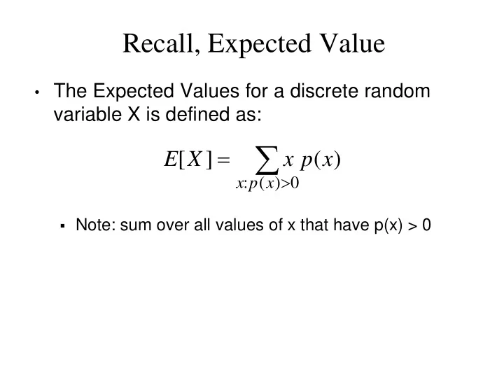

  1. Recall, Expected Value • The Expected Values for a discrete random variable X is defined as: ∑ = [ ] ( ) E X x p x > : ( ) 0 x p x  Note: sum over all values of x that have p(x) > 0

  2. The St. Petersburg Paradox • Game set-up  We have a fair coin (come up “heads” with p = 0.5)  Let n = number of coin flips (“heads”) before first “tails”  You win $2 n • How much would you pay to play? • Solution  Let X = your winnings. Claim: E[X] = ∞ + 1 2 3 1 ∞ i         1 1 1 1 ∑ + + + =         0 1 2 i Proof: E[X] = 2 2 2 ... 2         2 2 2 2 = 0 i ∞ 1 = ∑ = ∞ = 0 2 i  I’ll let you play for $1 million... but just once! Takers?

  3. Reminder of Geometric Series n ∑ + + + + + = 0 1 2 3 n i • Geometric series: ... x x x x x x = 0 i • A handy formula: − + n 1 n 1 ∑ x = i x − 1 x = i 0 • As n → ∞ , and | x | < 1, then − + n 1 n 1 1 ∑ x = → i x − − 1 1 x x = i 0

  4. Breaking Vegas • Consider even money bet (e.g., bet “Red” in roulette)  p = 18/38 you win bet, otherwise (1 – p) you lose bet  Consider this method for how to determine our bets: 1. Y = $1 2. Bet Y 3. If Win then STOP 4. If Loss then Y = 2 * Y, go to Step 2 Let Z = winnings upon stopping  Claim: E[Z] = 1  Here’s the proof in case you don’t believe me: o   ∞ i − ∞ i           1 i 20 18 18 20 18 1 ∑ ∑ ∑   = − = = =           i j E [ ] 2 2 1 Z             20 38 38   38 38 38 − = = = i 0 j 0 i 0 1 38 Expected winnings ≥ 0. Repeat process infinitely! 

  5. Vegas Breaks You • Why doesn’t everyone do this?  Real games have maximum bet amounts  You have finite money o Not able to keep doubling bet beyond certain point  Casinos can kick you out • But, if you had:  No betting limits, and  Infinite money, and  Could play as often as you want... • Then, go for it!  And tell me which planet you are living on

  6. Variance • Consider the following 3 distributions (PMFs) • All have the same expected value, E[X] = 3 • But “spread” in distributions is different • Variance = a formal quantification of “spread”

  7. Variance • If X is a random variable with mean µ then the variance of X , denoted Var( X ), is: Var( X ) = E [( X – µ ) 2 ]  Note: Var( X ) ≥ 0 • Often computed as: Var(X) = E[ X 2 ] – (E[X]) 2 • Standard Deviation of X, denoted SD(X), is: X = SD ( ) Var ( X )  Var(X) is in units of X 2  SD(X) is in same units as X

  8. Variance of 6 Sided Die • Let X = value on roll of 6 sided die • Recall that E[X] = 7/2 • Compute E[X 2 ] ( ) ( ) ( ) ( ) ( ) ( ) 1 1 1 1 1 1 91 = + + + + + = 2 2 2 2 2 2 2 [ ] 1 2 3 4 5 6 E X 6 6 6 6 6 6 6 = − 2 2 Var ( X ) E [ X ] ( E [ X ]) 2   91 7 35 = − =     6 2 12

  9. Jacob Bernoulli • Jacob Bernoulli (1654-1705), also known as “James”, was a Swiss mathematician • One of many mathematicians in Bernoulli family • The Bernoulli Random Variable is named for him • He is my academic great 11 -grandfather

  10. Bernoulli Random Variable • Experiment results in “Success” or “Failure”  X is random indicator variable (1 = success, 0 = failure)  P(X = 1) = p(1) = p P(X = 0) = p(0) = 1 – p  X is a Bernoulli Random Variable: X ~ Ber(p)  E[X] = p  Var(X) = p(1 – p) • Examples  coin flip  winning the lottery (p would be very small)

  11. Binomial Random Variable • Consider n independent trials of Ber(p) rand. var.  X is number of successes in n trials  X is a Binomial Random Variable: X ~ Bin(n, p)   n = = =   − − = i n i ( ) ( ) ( 1 ) 0 , 1 ,..., P X i p i   p p i n   i  E[X] = np  Var(X) = np(1 – p) • Examples  # of heads in n coin flips

  12. Three Coin Flips • Three fair (“heads” with p = 0.5) coins are flipped  X is number of heads  X ~ Bin(3, 0.5)   3 1   = = − = 0 3 P ( X 0 ) p ( 1 p )     0 8   3 3   = = − = 1 2 ( 1 ) ( 1 ) P X   p p   1 8   3 3   = = − = 2 1 ( 2 ) ( 1 ) P X   p p   2 8   3 1   = = − = 3 0 ( 3 ) ( 1 ) P X   p p   3 8

  13. PMF for X ~ Bin(10, 0.5) P(X=k) k

  14. PMF for X ~ Bin(10, 0.3) P(X=k) k

  15. Error Correcting Codes • Error correcting codes  Have original 4 bit string to send over network  Add 3 “parity” bits, and send 7 bits total  Each bit independently corrupted (flipped) in transition with probability 0.1  X = number of bits corrupted: X ~ Bin(7, 0.1)  But, parity bits allow us to correct at most 1 bit error • P(a correctable message is received)?  P(X = 0) + P(X = 1)

  16. Error Correcting Codes (cont) • Using error correcting codes: X ~ Bin(7, 0.1)   7   = = ≈ 0 7 P ( X 0 ) ( 0 . 1 ) ( 0 . 9 ) 0 . 4783     0   7   = = ≈ 1 6 ( 1 ) ( 0 . 1 ) ( 0 . 9 ) 0 . 3720 P X     1  P(X = 0) + P(X = 1) = 0.8503 • What if we didn’t use error correcting codes?  X ~ Bin(4, 0.1)  P(correct message received) = P(X = 0)   4   = = = 0 4 P ( X 0 ) ( 0 . 1 ) ( 0 . 9 ) 0 . 6561     0 • Using error correction improves reliability ~30%!

  17. Genetic Inheritance • Person has 2 genes for trait (eye color)  Child receives 1 gene (equally likely) from each parent  Child has brown eyes if either (or both) genes brown  Child only has blue eyes if both genes blue  Brown is “dominant” (d) , Blue is “recessive” (r)  Parents each have 1 brown and 1 blue gene • 4 children, what is P(3 children with brown eyes)?  Child has blue eyes: p = (½) (½) = ¼ (2 blue genes)  P(child has brown eyes) = 1 – (¼) = 0.75  X = # of children with brown eyes. X ~ Bin(4, 0.75)   4   = = ≈ 3 1 ( 3 ) ( 0 . 75 ) ( 0 . 25 ) 0 . 4219 P X     3

  18. Power of Your Vote • Is it better to vote in small or large state?  Small: more likely your vote changes outcome  Large: larger outcome (electoral votes) if state swings  a (= 2n) voters equally likely to vote for either candidate  You are deciding (a + 1) st vote   n n     2 n 1 1 ( 2 )! n =   =     ( 2 voters tie ) P n       2 n   n 2 2 n ! n ! 2 ≈ + − π 1 / 2 n n  Use Stirling’s Approximation: ! 2 n n e + − π 2 1 / 2 2 n n ( 2 ) 2 1 n e ≈ = ( 2 voters tie ) P n + − π π 2 1 2 2 n n n 2 2 n e n 1 2 c a = ( ) ac  Power = P(tie) * Elec. Votes = π π ( / 2 ) a  Larger state = more power

Download Presentation
Download Policy: The content available on the website is offered to you 'AS IS' for your personal information and use only. It cannot be commercialized, licensed, or distributed on other websites without prior consent from the author. To download a presentation, simply click this link. If you encounter any difficulties during the download process, it's possible that the publisher has removed the file from their server.

Recommend


More recommend