e.m. Field tensor & covariant equation of motion Define the - PowerPoint PPT Presentation

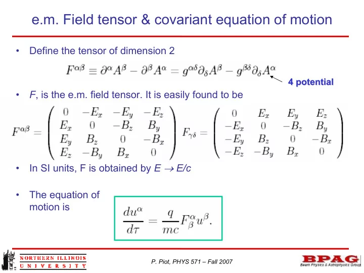
e.m. Field tensor & covariant equation of motion • Define the tensor of dimension 2 4 potential 4 potential • F , is the e.m. field tensor. It is easily found to be In SI units, F is obtained by E → E/c • • The equation of motion is P. Piot, PHYS 571 – Fall 2007

Invariant of the e.m. field tensor • Consider the following invariant quantities • Usually one redefine these invariants as • Which can be rewritten as where • Finally note the identities P. Piot, PHYS 571 – Fall 2007

Eigenvalues of the e.m. field tensor • The eigenvalues are given by • Characteristic polynomial • With solutions P. Piot, PHYS 571 – Fall 2007

Motion in an arbitrary e.m. field I • We now attempt to solve directly the equation We consider a time independent e.m. field following the treatment by Munos. Let • The equation of motion reduces to • Where the matrix exponential is defined as P. Piot, PHYS 571 – Fall 2007

Motion in an arbitrary e.m. field II • The main work is now to compute the matrix exponential. • To compute the power series of F one needs to recall the identities • Because of this one can show that any power of F can be written as linear combination of F, F , F 2 and I : • This means P. Piot, PHYS 571 – Fall 2007

Motion in an arbitrary e.m. field III • Consider . • We need to compute the coefficient of the expansion P. Piot, PHYS 571 – Fall 2007

Motion in an arbitrary e.m. field IV • The solution for the coefficient is . • Now let evaluate the t i ’s • The Trace is invariant upon change of basis. So consider a basis where F is diagonal, let F’ be the diagonal form then • Recall than P. Piot, PHYS 571 – Fall 2007

Motion in an arbitrary e.m. field V • The traces are then . • Now let evaluate the t i ’s P. Piot, PHYS 571 – Fall 2007

Motion in an arbitrary e.m. field VI • The traces are then . • Substitute in the power expansion to yield P. Piot, PHYS 571 – Fall 2007

Motion in an arbitrary e.m. field VII • Remember that • Integrate for P. Piot, PHYS 571 – Fall 2007

Motion in an arbitrary e.m. field VIII • Let’s consider the special case • Then • So we just take the limit in the equation motion derived in the previous slide which means: • So we obtain P. Piot, PHYS 571 – Fall 2007

ExB drift • With • compute P. Piot, PHYS 571 – Fall 2007

ExB drift I • With • compute P. Piot, PHYS 571 – Fall 2007

ExB drift II • The “projected” equation of motions • ….. • This is the so-called ExB drift and the drift velocity of the particle is P. Piot, PHYS 571 – Fall 2007

ExB drift III P. Piot, PHYS 571 – Fall 2007